

10 Layer Segmentation and Analysis for Retina with Diseases
249
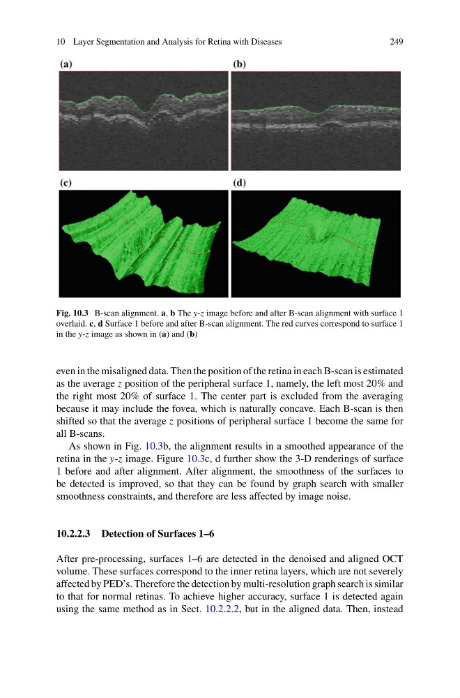
Fig. 10.3 B-scan alignment. a, b The y-z image before and after B-scan alignment with surface 1
overlaid. c, d Surface 1 before and after B-scan alignment. The red curves correspond to surface 1
in the y-z image as shown in (a) and (b)
even in the misaligned data. Then the position of the retina in each B-scan is estimated
as the average z position of the peripheral surface 1, namely, the left most 20% and
the right most 20% of surface 1. The center part is excluded from the averaging
because it may include the fovea, which is naturally concave. Each B-scan is then
shifted so that the average z positions of peripheral surface 1 become the same for
all B-scans.
As shown in Fig. 10.3b, the alignment results in a smoothed appearance of the
retina in the y-z image. Figure 10.3c, d further show the 3-D renderings of surface
1 before and after alignment. After alignment, the smoothness of the surfaces to
be detected is improved, so that they can be found by graph search with smaller
smoothness constraints, and therefore are less affected by image noise.
10.2.2.3 Detection of Surfaces 1–6
After pre-processing, surfaces 1–6 are detected in the denoised and aligned OCT
volume. These surfaces correspond to the inner retina layers, which are not severely
affected by PED’s. Therefore the detection by multi-resolution graph search is similar
to that for normal retinas. To achieve higher accuracy, surface 1 is detected again
using the same method as in Sect. 10.2.2.2, but in the aligned data. Then, instead
249
Fig. 10.3 B-scan alignment. a, b The y-z image before and after B-scan alignment with surface 1
overlaid. c, d Surface 1 before and after B-scan alignment. The red curves correspond to surface 1
in the y-z image as shown in (a) and (b)
even in the misaligned data. Then the position of the retina in each B-scan is estimated
as the average z position of the peripheral surface 1, namely, the left most 20% and
the right most 20% of surface 1. The center part is excluded from the averaging
because it may include the fovea, which is naturally concave. Each B-scan is then
shifted so that the average z positions of peripheral surface 1 become the same for
all B-scans.
As shown in Fig. 10.3b, the alignment results in a smoothed appearance of the
retina in the y-z image. Figure 10.3c, d further show the 3-D renderings of surface
1 before and after alignment. After alignment, the smoothness of the surfaces to
be detected is improved, so that they can be found by graph search with smaller
smoothness constraints, and therefore are less affected by image noise.
10.2.2.3 Detection of Surfaces 1–6
After pre-processing, surfaces 1–6 are detected in the denoised and aligned OCT
volume. These surfaces correspond to the inner retina layers, which are not severely
affected by PED’s. Therefore the detection by multi-resolution graph search is similar
to that for normal retinas. To achieve higher accuracy, surface 1 is detected again
using the same method as in Sect. 10.2.2.2, but in the aligned data. Then, instead