

9 Choroidal OCT Analytics
229
where we optimize the center (X c , Y c , Z c ) and radius R of the nominal sphere,
denoting Φ = {X c , Y c , Z c , R} for convenience, jointly with the free planar transformation parameters Ψ = (α i , β i , γ i )
K−1
i=2 .
C. Optimal planar transformations: The optimal choice of Ψ
∗ in (9.10) specifies the
collection of optimal planar transformations T i , 2 ≤ i ≤ K − 1. So, in order to
achieve spherical alignment, it is tempting to simply transform the i-th preprocessed section, 2 ≤ i ≤ K − 1. However, this method generally maps a point on
the integer grid to a point that does not lie on the integer grid on the transformed
axes. Appropriate interpolation will be performed to obtain image values on the
desired integer grid.
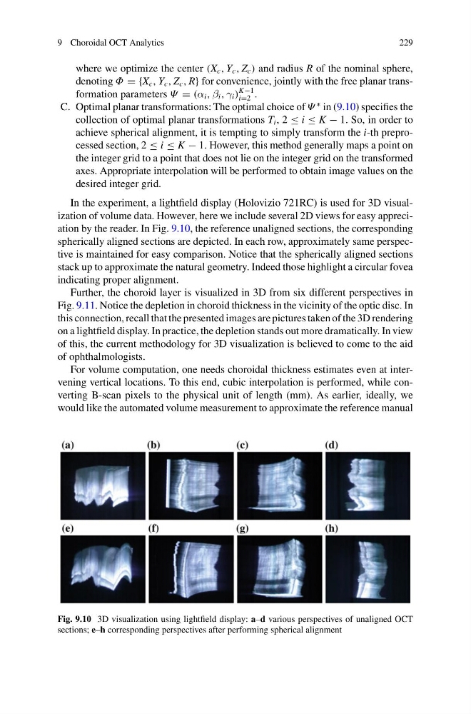
In the experiment, a lightfield display (Holovizio 721RC) is used for 3D visualization of volume data. However, here we include several 2D views for easy appreciation by the reader. In Fig. 9.10, the reference unaligned sections, the corresponding
spherically aligned sections are depicted. In each row, approximately same perspective is maintained for easy comparison. Notice that the spherically aligned sections
stack up to approximate the natural geometry. Indeed those highlight a circular fovea
indicating proper alignment.
Further, the choroid layer is visualized in 3D from six different perspectives in
Fig. 9.11. Notice the depletion in choroid thickness in the vicinity of the optic disc. In
this connection, recall that the presented images are pictures taken of the 3D rendering
on a lightfield display. In practice, the depletion stands out more dramatically. In view
of this, the current methodology for 3D visualization is believed to come to the aid
of ophthalmologists.
For volume computation, one needs choroidal thickness estimates even at intervening vertical locations. To this end, cubic interpolation is performed, while converting B-scan pixels to the physical unit of length (mm). As earlier, ideally, we
would like the automated volume measurement to approximate the reference manual
Fig. 9.10 3D visualization using lightfield display: a–d various perspectives of unaligned OCT
sections; e–h corresponding perspectives after performing spherical alignment
229
where we optimize the center (X c , Y c , Z c ) and radius R of the nominal sphere,
denoting Φ = {X c , Y c , Z c , R} for convenience, jointly with the free planar transformation parameters Ψ = (α i , β i , γ i )
K−1
i=2 .
C. Optimal planar transformations: The optimal choice of Ψ
∗ in (9.10) specifies the
collection of optimal planar transformations T i , 2 ≤ i ≤ K − 1. So, in order to
achieve spherical alignment, it is tempting to simply transform the i-th preprocessed section, 2 ≤ i ≤ K − 1. However, this method generally maps a point on
the integer grid to a point that does not lie on the integer grid on the transformed
axes. Appropriate interpolation will be performed to obtain image values on the
desired integer grid.
In the experiment, a lightfield display (Holovizio 721RC) is used for 3D visualization of volume data. However, here we include several 2D views for easy appreciation by the reader. In Fig. 9.10, the reference unaligned sections, the corresponding
spherically aligned sections are depicted. In each row, approximately same perspective is maintained for easy comparison. Notice that the spherically aligned sections
stack up to approximate the natural geometry. Indeed those highlight a circular fovea
indicating proper alignment.
Further, the choroid layer is visualized in 3D from six different perspectives in
Fig. 9.11. Notice the depletion in choroid thickness in the vicinity of the optic disc. In
this connection, recall that the presented images are pictures taken of the 3D rendering
on a lightfield display. In practice, the depletion stands out more dramatically. In view
of this, the current methodology for 3D visualization is believed to come to the aid
of ophthalmologists.
For volume computation, one needs choroidal thickness estimates even at intervening vertical locations. To this end, cubic interpolation is performed, while converting B-scan pixels to the physical unit of length (mm). As earlier, ideally, we
would like the automated volume measurement to approximate the reference manual
Fig. 9.10 3D visualization using lightfield display: a–d various perspectives of unaligned OCT
sections; e–h corresponding perspectives after performing spherical alignment