

5 Segmentation of OCT Scans Using Probabilistic Graphical Models
111
where we used Bayes theorem [22, Eq. (A.3)] to equate
p(y|c) p(c)
p(y)
with p(c|y). Since
p(b) already contains prior knowledge about the shape of boundary positions, we
assume an uninformative prior for c. Hence dropping p(c) and taking into account
the factorization of q, (5.11) results in the objective function
J (q b , q c ) = −
b
c
q b (b)q c (c) log
p(c|y) p(c|b) p(b)
db − H [q b ] − H [q c ],
(5.12)
where H [q b ] and H [q c ] are the entropies of q b and q c .
Definitions of q c and q b . For q c we adopt the structure of p(c|b), that is, written in
a slightly different but equivalent form
q c (c) =
M
j=1
q c (c 1, j )
K
k=2
q c (c k, j , c k−1, j )
q c (c k−1, j )
.
(5.13)
For q b we adopt the Gaussian model of b
q b (b) = N (b; ¯
μ, ),
(5.14)
where the bar-notation distinguishes the parameters of q b from those of p(b).
Explicit Form of J(q b , q c ). Direct optimization of the objective (5.12) requires to
sum over all combinations of c and integrating over b, and therefore is intractable
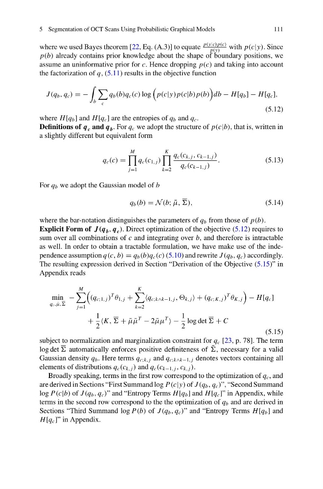
as well. In order to obtain a tractable formulation, we have make use of the independence assumption q(c, b) = q b (b)q c (c) (5.10) and rewrite J (q b , q c ) accordingly.
The resulting expression derived in Section “Derivation of the Objective (5.15)” in
Appendix reads
min
q c , ¯
μ,
−
M
j=1
(q c;1, j )
T
θ 1, j +
K
k=2
q c;k∧k−1, j , , k, j + (q c;K , j )
T
θ K , j
− H [q c ]
+
1
2
K , + ¯
μ ¯
μ
T
− 2 ¯
μμ
T
−
1
2
log det + C
(5.15)
subject to normalization and marginalization constraint for q c [23, p. 78]. The term
log det automatically enforces positive definiteness of ¯
, necessary for a valid
Gaussian density q b . Here terms q c;k, j and q c;k∧k−1, j denotes vectors containing all
elements of distributions q c (c k, j ) and q c (c k−1, j , c k, j ).
Broadly speaking, terms in the first row correspond to the optimization of q c , and
are derived in Sections “First Summand log P(c|y) of J (q b , q c )”, “Second Summand
log P(c|b) of J (q b , q c )” and “Entropy Terms H [q b ] and H [q c ]” in Appendix, while
terms in the second row correspond to the the optimization of q b and are derived in
Sections “Third Summand log P(b) of J (q b , q c )” and “Entropy Terms H [q b ] and
H [q c ]” in Appendix.
111
where we used Bayes theorem [22, Eq. (A.3)] to equate
p(y|c) p(c)
p(y)
with p(c|y). Since
p(b) already contains prior knowledge about the shape of boundary positions, we
assume an uninformative prior for c. Hence dropping p(c) and taking into account
the factorization of q, (5.11) results in the objective function
J (q b , q c ) = −
b
c
q b (b)q c (c) log
p(c|y) p(c|b) p(b)
db − H [q b ] − H [q c ],
(5.12)
where H [q b ] and H [q c ] are the entropies of q b and q c .
Definitions of q c and q b . For q c we adopt the structure of p(c|b), that is, written in
a slightly different but equivalent form
q c (c) =
M
j=1
q c (c 1, j )
K
k=2
q c (c k, j , c k−1, j )
q c (c k−1, j )
.
(5.13)
For q b we adopt the Gaussian model of b
q b (b) = N (b; ¯
μ, ),
(5.14)
where the bar-notation distinguishes the parameters of q b from those of p(b).
Explicit Form of J(q b , q c ). Direct optimization of the objective (5.12) requires to
sum over all combinations of c and integrating over b, and therefore is intractable
as well. In order to obtain a tractable formulation, we have make use of the independence assumption q(c, b) = q b (b)q c (c) (5.10) and rewrite J (q b , q c ) accordingly.
The resulting expression derived in Section “Derivation of the Objective (5.15)” in
Appendix reads
min
q c , ¯
μ,
−
M
j=1
(q c;1, j )
T
θ 1, j +
K
k=2
q c;k∧k−1, j , , k, j + (q c;K , j )
T
θ K , j
− H [q c ]
+
1
2
K , + ¯
μ ¯
μ
T
− 2 ¯
μμ
T
−
1
2
log det + C
(5.15)
subject to normalization and marginalization constraint for q c [23, p. 78]. The term
log det automatically enforces positive definiteness of ¯
, necessary for a valid
Gaussian density q b . Here terms q c;k, j and q c;k∧k−1, j denotes vectors containing all
elements of distributions q c (c k, j ) and q c (c k−1, j , c k, j ).
Broadly speaking, terms in the first row correspond to the optimization of q c , and
are derived in Sections “First Summand log P(c|y) of J (q b , q c )”, “Second Summand
log P(c|b) of J (q b , q c )” and “Entropy Terms H [q b ] and H [q c ]” in Appendix, while
terms in the second row correspond to the the optimization of q b and are derived in
Sections “Third Summand log P(b) of J (q b , q c )” and “Entropy Terms H [q b ] and
H [q c ]” in Appendix.