

110
F. Rathke et al.
As a result the communication across image columns is induced not by the structure of the Markov random field but by the definition of its marginal distributions, conditioning on b \ j . While the definition (5.8) does not take the ordering constraint (5.2)
into account, this is done during inference (Section “Second Summand log P(c|b)
of J (q b , q c )” in Appendix).
2-D versus 3-D. Our description so far considered OCT scans of dimension two.
Nevertheless, our approach is equally applicable to 3-D volumes. We use the very
same notation, since adding additional B-Scans will only increase the number of
image columns M. Similarly, the connectivity of the graphical model p(y, c, b) can
be transferred one-to-one.
5.2.2 Variational Inference
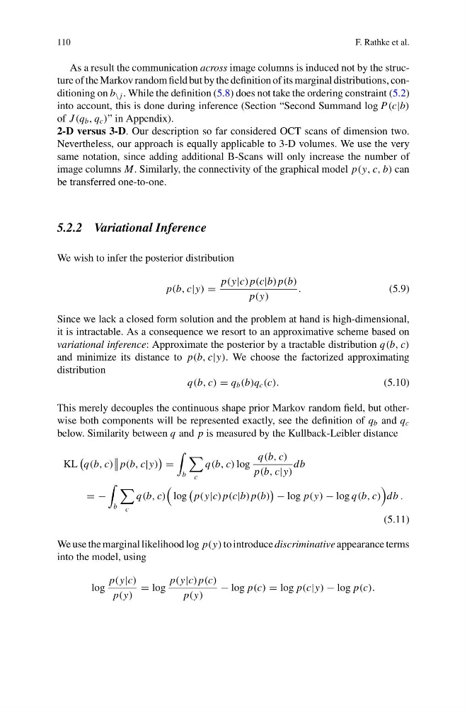
We wish to infer the posterior distribution
p(b, c|y) =
p(y|c) p(c|b) p(b)
p(y)
.
(5.9)
Since we lack a closed form solution and the problem at hand is high-dimensional,
it is intractable. As a consequence we resort to an approximative scheme based on
variational inference: Approximate the posterior by a tractable distribution q(b, c)
and minimize its distance to p(b, c|y). We choose the factorized approximating
distribution
q(b, c) = q b (b)q c (c).
(5.10)
This merely decouples the continuous shape prior Markov random field, but otherwise both components will be represented exactly, see the definition of q b and q c
below. Similarity between q and p is measured by the Kullback-Leibler distance
KL
q(b, c)
p(b, c|y)
=
b
c
q(b, c) log
q(b, c)
p(b, c|y)
db
= −
b
c
q(b, c)
log
p(y|c) p(c|b) p(b)
− log p(y) − log q(b, c)
db .
(5.11)
We use the marginal likelihood log p(y) to introduce discriminative appearance terms
into the model, using
log
p(y|c)
p(y)
= log
p(y|c) p(c)
p(y)
− log p(c) = log p(c|y) − log p(c).
F. Rathke et al.
As a result the communication across image columns is induced not by the structure of the Markov random field but by the definition of its marginal distributions, conditioning on b \ j . While the definition (5.8) does not take the ordering constraint (5.2)
into account, this is done during inference (Section “Second Summand log P(c|b)
of J (q b , q c )” in Appendix).
2-D versus 3-D. Our description so far considered OCT scans of dimension two.
Nevertheless, our approach is equally applicable to 3-D volumes. We use the very
same notation, since adding additional B-Scans will only increase the number of
image columns M. Similarly, the connectivity of the graphical model p(y, c, b) can
be transferred one-to-one.
5.2.2 Variational Inference
We wish to infer the posterior distribution
p(b, c|y) =
p(y|c) p(c|b) p(b)
p(y)
.
(5.9)
Since we lack a closed form solution and the problem at hand is high-dimensional,
it is intractable. As a consequence we resort to an approximative scheme based on
variational inference: Approximate the posterior by a tractable distribution q(b, c)
and minimize its distance to p(b, c|y). We choose the factorized approximating
distribution
q(b, c) = q b (b)q c (c).
(5.10)
This merely decouples the continuous shape prior Markov random field, but otherwise both components will be represented exactly, see the definition of q b and q c
below. Similarity between q and p is measured by the Kullback-Leibler distance
KL
q(b, c)
p(b, c|y)
=
b
c
q(b, c) log
q(b, c)
p(b, c|y)
db
= −
b
c
q(b, c)
log
p(y|c) p(c|b) p(b)
− log p(y) − log q(b, c)
db .
(5.11)
We use the marginal likelihood log p(y) to introduce discriminative appearance terms
into the model, using
log
p(y|c)
p(y)
= log
p(y|c) p(c)
p(y)
− log p(c) = log p(c|y) − log p(c).