

5 Segmentation of OCT Scans Using Probabilistic Graphical Models
109
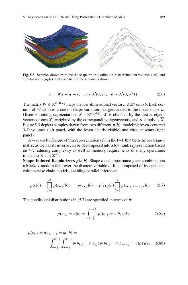
Fig. 5.3 Samples drawn from the the shape prior distribution p(b) trained on volumes (left) and
circular scans (right). Only one half of the volume is shown
b = W s + μ + s ∼ N (0, I ), , ∼ N (0, σ
2 I ).
(5.6)
The matrix W ∈ R
K ·M×q maps the low-dimensional vector s ∈ R
q onto b. Each column of W denotes a certain shape variation that gets added to the mean shape μ.
Given n training segmentations X ∈ R
n×M·K , W is obtained by the first m eigenvectors of cov(X ) weighted by the corresponding eigenvectors, and μ simply is X .
Figure 5.3 depicts samples drawn from two different p(b), modeling fovea-centered
3-D volumes (left panel, with the fovea clearly visible) and circular scans (right
panel).
A very useful feature of this representation of b is the fact, that both the covariance
matrix as well as its inverse can be decomposed into a low-rank representation based
on W , reducing complexity as well as memory requirements of many operations
related to and
−1 .
Shape-Induced Regularizers p(c|b). Shape b and appearance y are combined via
a Markov random field over the discrete variable c. It is composed of independent
column-wise chain models, enabling parallel inference:
p(c|b) =
M
j=1
p(c •, j |b),
p(c •, j |b) = p(c 1, j |b)
K
k=2
p(c k, j |c k−1, j , b).
(5.7)
The conditional distributions in (5.7) are specified in terms of b:
p(c 1, j = n|b) =
n+
1
2
n−
1
2
p(b 1, j = τ |b \ j )dτ,
(5.8a)
p(c k, j = n|c k−1, j = m, b) =
n+
1
2
n−
1
2
m+
1
2
m−
1
2
p(b k, j = τ |b \ j ) p(b k, j = τ |b k−1, j = ν)dτ dν. (5.8b)
109
Fig. 5.3 Samples drawn from the the shape prior distribution p(b) trained on volumes (left) and
circular scans (right). Only one half of the volume is shown
b = W s + μ + s ∼ N (0, I ), , ∼ N (0, σ
2 I ).
(5.6)
The matrix W ∈ R
K ·M×q maps the low-dimensional vector s ∈ R
q onto b. Each column of W denotes a certain shape variation that gets added to the mean shape μ.
Given n training segmentations X ∈ R
n×M·K , W is obtained by the first m eigenvectors of cov(X ) weighted by the corresponding eigenvectors, and μ simply is X .
Figure 5.3 depicts samples drawn from two different p(b), modeling fovea-centered
3-D volumes (left panel, with the fovea clearly visible) and circular scans (right
panel).
A very useful feature of this representation of b is the fact, that both the covariance
matrix as well as its inverse can be decomposed into a low-rank representation based
on W , reducing complexity as well as memory requirements of many operations
related to and
−1 .
Shape-Induced Regularizers p(c|b). Shape b and appearance y are combined via
a Markov random field over the discrete variable c. It is composed of independent
column-wise chain models, enabling parallel inference:
p(c|b) =
M
j=1
p(c •, j |b),
p(c •, j |b) = p(c 1, j |b)
K
k=2
p(c k, j |c k−1, j , b).
(5.7)
The conditional distributions in (5.7) are specified in terms of b:
p(c 1, j = n|b) =
n+
1
2
n−
1
2
p(b 1, j = τ |b \ j )dτ,
(5.8a)
p(c k, j = n|c k−1, j = m, b) =
n+
1
2
n−
1
2
m+
1
2
m−
1
2
p(b k, j = τ |b \ j ) p(b k, j = τ |b k−1, j = ν)dτ dν. (5.8b)