

20.3.5
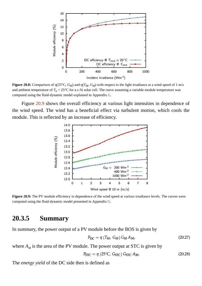
Figure 20.8: Comparison of η(25°C, G M ) and η(T M , G M ) with respect to the light irradiance at a wind speed of 1 m/s
and ambient temperature of T a = 25°C for a c-Si solar cell. The curve assuming a variable module temperature was
computed using the fluid-dynamic model explained in Appendix G.
Figure 20.9 shows the overall efficiency at various light intensities in dependence of
the wind speed. The wind has a beneficial effect via turbulent motion, which cools the
module. This is reflected by an increase of efficiency.
Figure 20.9: The PV module efficiency in dependence of the wind speed at various irradiance levels. The curves were
computed using the fluid-dynamic model presented in Appendix G.
Summary
In summary, the power output of a PV module before the BOS is given by
where A M is the area of the PV module. The power output at STC is given by
The energy yield of the DC side then is defined as
Figure 20.8: Comparison of η(25°C, G M ) and η(T M , G M ) with respect to the light irradiance at a wind speed of 1 m/s
and ambient temperature of T a = 25°C for a c-Si solar cell. The curve assuming a variable module temperature was
computed using the fluid-dynamic model explained in Appendix G.
Figure 20.9 shows the overall efficiency at various light intensities in dependence of
the wind speed. The wind has a beneficial effect via turbulent motion, which cools the
module. This is reflected by an increase of efficiency.
Figure 20.9: The PV module efficiency in dependence of the wind speed at various irradiance levels. The curves were
computed using the fluid-dynamic model presented in Appendix G.
Summary
In summary, the power output of a PV module before the BOS is given by
where A M is the area of the PV module. The power output at STC is given by
The energy yield of the DC side then is defined as