

A
B
C
Note
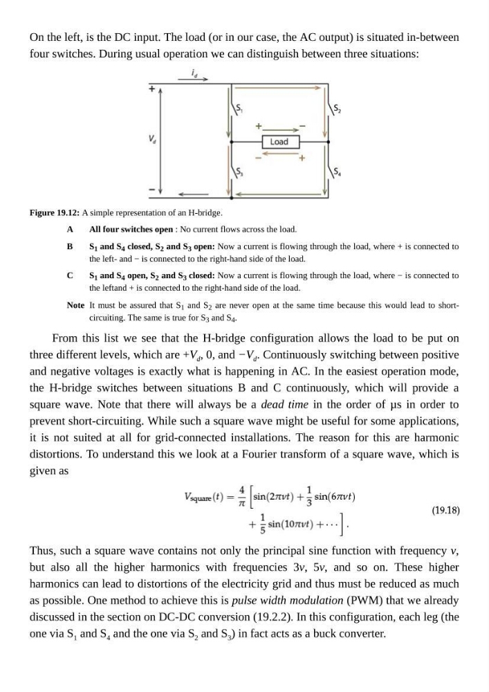
On the left, is the DC input. The load (or in our case, the AC output) is situated in-between
four switches. During usual operation we can distinguish between three situations:
Figure 19.12: A simple representation of an H-bridge.
All four switches open : No current flows across the load.
S 1 and S 4 closed, S 2 and S 3 open: Now a current is flowing through the load, where + is connected to
the left- and − is connected to the right-hand side of the load.
S 1 and S 4 open, S 2 and S 3 closed: Now a current is flowing through the load, where − is connected to
the leftand + is connected to the right-hand side of the load.
It must be assured that S 1 and S 2 are never open at the same time because this would lead to shortcircuiting. The same is true for S 3 and S 4 .
From this list we see that the H-bridge configuration allows the load to be put on
three different levels, which are +V d , 0, and −V d . Continuously switching between positive
and negative voltages is exactly what is happening in AC. In the easiest operation mode,
the H-bridge switches between situations B and C continuously, which will provide a
square wave. Note that there will always be a dead time in the order of µs in order to
prevent short-circuiting. While such a square wave might be useful for some applications,
it is not suited at all for grid-connected installations. The reason for this are harmonic
distortions. To understand this we look at a Fourier transform of a square wave, which is
given as
Thus, such a square wave contains not only the principal sine function with frequency ν,
but also all the higher harmonics with frequencies 3ν, 5ν, and so on. These higher
harmonics can lead to distortions of the electricity grid and thus must be reduced as much
as possible. One method to achieve this is pulse width modulation (PWM) that we already
discussed in the section on DC-DC conversion (19.2.2). In this configuration, each leg (the
one via S 1 and S 4 and the one via S 2 and S 3 ) in fact acts as a buck converter.
B
C
Note
On the left, is the DC input. The load (or in our case, the AC output) is situated in-between
four switches. During usual operation we can distinguish between three situations:
Figure 19.12: A simple representation of an H-bridge.
All four switches open : No current flows across the load.
S 1 and S 4 closed, S 2 and S 3 open: Now a current is flowing through the load, where + is connected to
the left- and − is connected to the right-hand side of the load.
S 1 and S 4 open, S 2 and S 3 closed: Now a current is flowing through the load, where − is connected to
the leftand + is connected to the right-hand side of the load.
It must be assured that S 1 and S 2 are never open at the same time because this would lead to shortcircuiting. The same is true for S 3 and S 4 .
From this list we see that the H-bridge configuration allows the load to be put on
three different levels, which are +V d , 0, and −V d . Continuously switching between positive
and negative voltages is exactly what is happening in AC. In the easiest operation mode,
the H-bridge switches between situations B and C continuously, which will provide a
square wave. Note that there will always be a dead time in the order of µs in order to
prevent short-circuiting. While such a square wave might be useful for some applications,
it is not suited at all for grid-connected installations. The reason for this are harmonic
distortions. To understand this we look at a Fourier transform of a square wave, which is
given as
Thus, such a square wave contains not only the principal sine function with frequency ν,
but also all the higher harmonics with frequencies 3ν, 5ν, and so on. These higher
harmonics can lead to distortions of the electricity grid and thus must be reduced as much
as possible. One method to achieve this is pulse width modulation (PWM) that we already
discussed in the section on DC-DC conversion (19.2.2). In this configuration, each leg (the
one via S 1 and S 4 and the one via S 2 and S 3 ) in fact acts as a buck converter.