

Negative
Positive
Negative
Negative
Negative
Positive
A problem with this algorithm is that the operating point is never steady at the MPP
but is meandering around the MPP. If very small perturbation steps are used around the
MPP, this meandering, however, can be minimized. Additionally, the P&O algorithm
struggles from rapidly changing illuminations. For example, if the illumination (and hence
the irradiance) changes in-between two sampling instants in the process of convergence,
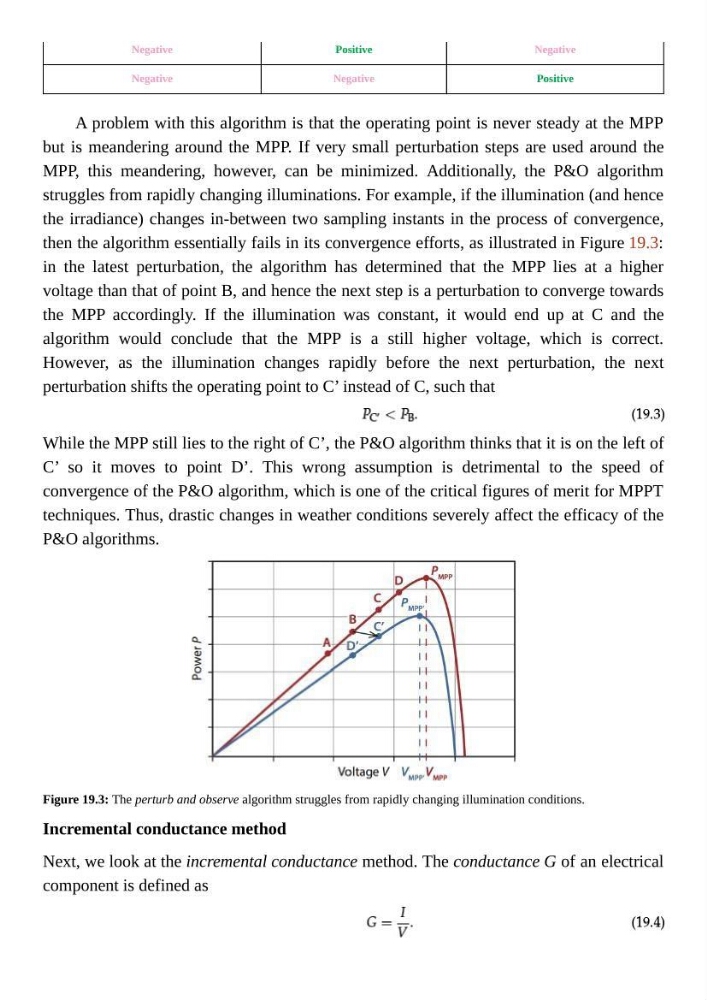
then the algorithm essentially fails in its convergence efforts, as illustrated in Figure 19.3:
in the latest perturbation, the algorithm has determined that the MPP lies at a higher
voltage than that of point B, and hence the next step is a perturbation to converge towards
the MPP accordingly. If the illumination was constant, it would end up at C and the
algorithm would conclude that the MPP is a still higher voltage, which is correct.
However, as the illumination changes rapidly before the next perturbation, the next
perturbation shifts the operating point to C’ instead of C, such that
While the MPP still lies to the right of C’, the P&O algorithm thinks that it is on the left of
C’ so it moves to point D’. This wrong assumption is detrimental to the speed of
convergence of the P&O algorithm, which is one of the critical figures of merit for MPPT
techniques. Thus, drastic changes in weather conditions severely affect the efficacy of the
P&O algorithms.
Figure 19.3: The perturb and observe algorithm struggles from rapidly changing illumination conditions.
Incremental conductance method
Next, we look at the incremental conductance method. The conductance G of an electrical
component is defined as
Positive
Negative
Negative
Negative
Positive
A problem with this algorithm is that the operating point is never steady at the MPP
but is meandering around the MPP. If very small perturbation steps are used around the
MPP, this meandering, however, can be minimized. Additionally, the P&O algorithm
struggles from rapidly changing illuminations. For example, if the illumination (and hence
the irradiance) changes in-between two sampling instants in the process of convergence,
then the algorithm essentially fails in its convergence efforts, as illustrated in Figure 19.3:
in the latest perturbation, the algorithm has determined that the MPP lies at a higher
voltage than that of point B, and hence the next step is a perturbation to converge towards
the MPP accordingly. If the illumination was constant, it would end up at C and the
algorithm would conclude that the MPP is a still higher voltage, which is correct.
However, as the illumination changes rapidly before the next perturbation, the next
perturbation shifts the operating point to C’ instead of C, such that
While the MPP still lies to the right of C’, the P&O algorithm thinks that it is on the left of
C’ so it moves to point D’. This wrong assumption is detrimental to the speed of
convergence of the P&O algorithm, which is one of the critical figures of merit for MPPT
techniques. Thus, drastic changes in weather conditions severely affect the efficacy of the
P&O algorithms.
Figure 19.3: The perturb and observe algorithm struggles from rapidly changing illumination conditions.
Incremental conductance method
Next, we look at the incremental conductance method. The conductance G of an electrical
component is defined as