

416
E. J. Brändas
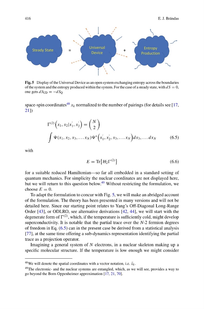
Fig. 5 Display of the Universal Device as an open system exchanging entropy across the boundaries
of the system and the entropy produced within the system. For the case of a steady state, with d S = 0,
one gets d S UD = −d S Q
space-spin coordinates
48 x k normalized to the number of pairings (for details see [17,
21])
(2)
x 1 , x 2 |x
1 , x
2
=
N
2
(x 1 , x 2 , x 3 , . . . x N )
∗
x
1 , x
2 , x 3 , . . . x N
dx 3 , . . . dx N
(6.5)
with
E = Tr
H 2
(2)
(6.6)
for a suitable reduced Hamiltonian—so far all embedded in a standard setting of
quantum mechanics. For simplicity the nuclear coordinates are not displayed here,
but we will return to this question below.
49 Without restricting the formulation, we
choose E = 0.
To adapt the formulation to concur with Fig. 5, we will make an abridged account
of the formulation. The theory has been presented in many versions and will not be
detailed here. Since our starting point relates to Yang’s Off-Diagonal Long-Range
Order [43], or ODLRO, see alternative derivations [42, 44], we will start with the
degenerate form of
(2) , which, if the temperature is sufficiently cold, might develop
superconductivity. It is notable that the partial trace over the N-2 fermion degrees
of freedom in Eq. (6.5) can in the present case be derived from a statistical analysis
[77], at the same time offering a sub-dynamics representation identifying the partial
trace as a projection operator.
Imagining a general system of N electrons, in a nuclear skeleton making up a
specific molecular structure. If the temperature is low enough we might consider
48 We will denote the spatial coordinates with a vector notation, i.e.
x k .
49 The electronic- and the nuclear systems are entangled, which, as we will see, provides a way to
go beyond the Born-Oppenheimer approximation [17, 21, 70].
E. J. Brändas
Fig. 5 Display of the Universal Device as an open system exchanging entropy across the boundaries
of the system and the entropy produced within the system. For the case of a steady state, with d S = 0,
one gets d S UD = −d S Q
space-spin coordinates
48 x k normalized to the number of pairings (for details see [17,
21])
(2)
x 1 , x 2 |x
1 , x
2
=
N
2
(x 1 , x 2 , x 3 , . . . x N )
∗
x
1 , x
2 , x 3 , . . . x N
dx 3 , . . . dx N
(6.5)
with
E = Tr
H 2
(2)
(6.6)
for a suitable reduced Hamiltonian—so far all embedded in a standard setting of
quantum mechanics. For simplicity the nuclear coordinates are not displayed here,
but we will return to this question below.
49 Without restricting the formulation, we
choose E = 0.
To adapt the formulation to concur with Fig. 5, we will make an abridged account
of the formulation. The theory has been presented in many versions and will not be
detailed here. Since our starting point relates to Yang’s Off-Diagonal Long-Range
Order [43], or ODLRO, see alternative derivations [42, 44], we will start with the
degenerate form of
(2) , which, if the temperature is sufficiently cold, might develop
superconductivity. It is notable that the partial trace over the N-2 fermion degrees
of freedom in Eq. (6.5) can in the present case be derived from a statistical analysis
[77], at the same time offering a sub-dynamics representation identifying the partial
trace as a projection operator.
Imagining a general system of N electrons, in a nuclear skeleton making up a
specific molecular structure. If the temperature is low enough we might consider
48 We will denote the spatial coordinates with a vector notation, i.e.
x k .
49 The electronic- and the nuclear systems are entangled, which, as we will see, provides a way to
go beyond the Born-Oppenheimer approximation [17, 21, 70].