

408
E. J. Brändas
second law says d S ≥ 0 and d S Q ≥ 0 implying d S UD ≥ −d S Q . The UD condition
thus becomes d S < d S Q . In particular the steady state condition, d S = 0, implies
d S UD = −d S Q , which is negative as long as any entropy production subsists. We will
preferentially refer to QM processes, since pure CM studies of conceivable UD’s may
yield different answers, see e.g. the analysis of the Cyclotron Maser Concept, CMC,
in [57]. The QM view will be shown to be crucial, while making a profound derivation
of the characteristics of our Universal Device. The relation with Schrödinger’s classic
treatment “What is Life?” and the practice of the associated concept of negentropy
is deferred to the Conclusion.
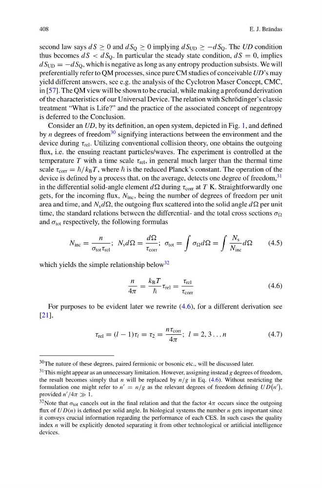
Consider an UD, by its definition, an open system, depicted in Fig. 1, and defined
by n degrees of freedom
30 signifying interactions between the environment and the
device during τ rel . Utilizing conventional collision theory, one obtains the outgoing
flux, i.e. the ensuing reactant particles/waves. The experiment is controlled at the
temperature T with a time scale τ rel , in general much larger than the thermal time
scale τ corr = /k B T , where is the reduced Planck’s constant. The operation of the
device is defined by a process that, on the average, detects one degree of freedom,
31
in the differential solid-angle element d during τ corr at T K. Straightforwardly one
gets, for the incoming flux, N inc , being the number of degrees of freedom per unit
area and time, and N s d, the outgoing flux scattered into the solid angle d per unit
time, the standard relations between the differential- and the total cross sections σ
and σ tot respectively, the following formulas
N inc =
n
σ tot τ rel
; N s d =
d
τ corr
; σ tot =
σ d =
N s
N inc
d
(4.5)
which yields the simple relationship below
32
n
4π
=
k B T
τ rel =
τ rel
τ corr
(4.6)
For purposes to be evident later we rewrite (4.6), for a different derivation see
[21],
τ rel = (l − 1)τ l = τ 2 =
nτ corr
4π
; l = 2, 3 . . . n
(4.7)
30 The nature of these degrees, paired fermionic or bosonic etc., will be discussed later.
31 This might appear as an unnecessary limitation. However, assigning instead g degrees of freedom,
the result becomes simply that n will be replaced by n/g in Eq. (4.6). Without restricting the
formulation one might refer to n = n/g as the relevant degrees of freedom defining U D
n
,
provided n /4π 1.
32 Note that σ tot cancels out in the final relation and that the factor 4π occurs since the outgoing
flux of U D(n) is defined per solid angle. In biological systems the number n gets important since
it conveys crucial information regarding the performance of each CES. In such cases the quality
index n will be explicitly denoted separating it from other technological or artificial intelligence
devices.
E. J. Brändas
second law says d S ≥ 0 and d S Q ≥ 0 implying d S UD ≥ −d S Q . The UD condition
thus becomes d S < d S Q . In particular the steady state condition, d S = 0, implies
d S UD = −d S Q , which is negative as long as any entropy production subsists. We will
preferentially refer to QM processes, since pure CM studies of conceivable UD’s may
yield different answers, see e.g. the analysis of the Cyclotron Maser Concept, CMC,
in [57]. The QM view will be shown to be crucial, while making a profound derivation
of the characteristics of our Universal Device. The relation with Schrödinger’s classic
treatment “What is Life?” and the practice of the associated concept of negentropy
is deferred to the Conclusion.
Consider an UD, by its definition, an open system, depicted in Fig. 1, and defined
by n degrees of freedom
30 signifying interactions between the environment and the
device during τ rel . Utilizing conventional collision theory, one obtains the outgoing
flux, i.e. the ensuing reactant particles/waves. The experiment is controlled at the
temperature T with a time scale τ rel , in general much larger than the thermal time
scale τ corr = /k B T , where is the reduced Planck’s constant. The operation of the
device is defined by a process that, on the average, detects one degree of freedom,
31
in the differential solid-angle element d during τ corr at T K. Straightforwardly one
gets, for the incoming flux, N inc , being the number of degrees of freedom per unit
area and time, and N s d, the outgoing flux scattered into the solid angle d per unit
time, the standard relations between the differential- and the total cross sections σ
and σ tot respectively, the following formulas
N inc =
n
σ tot τ rel
; N s d =
d
τ corr
; σ tot =
σ d =
N s
N inc
d
(4.5)
which yields the simple relationship below
32
n
4π
=
k B T
τ rel =
τ rel
τ corr
(4.6)
For purposes to be evident later we rewrite (4.6), for a different derivation see
[21],
τ rel = (l − 1)τ l = τ 2 =
nτ corr
4π
; l = 2, 3 . . . n
(4.7)
30 The nature of these degrees, paired fermionic or bosonic etc., will be discussed later.
31 This might appear as an unnecessary limitation. However, assigning instead g degrees of freedom,
the result becomes simply that n will be replaced by n/g in Eq. (4.6). Without restricting the
formulation one might refer to n = n/g as the relevant degrees of freedom defining U D
n
,
provided n /4π 1.
32 Note that σ tot cancels out in the final relation and that the factor 4π occurs since the outgoing
flux of U D(n) is defined per solid angle. In biological systems the number n gets important since
it conveys crucial information regarding the performance of each CES. In such cases the quality
index n will be explicitly denoted separating it from other technological or artificial intelligence
devices.