

Abiogenesis and the Second Law of Thermodynamics
409
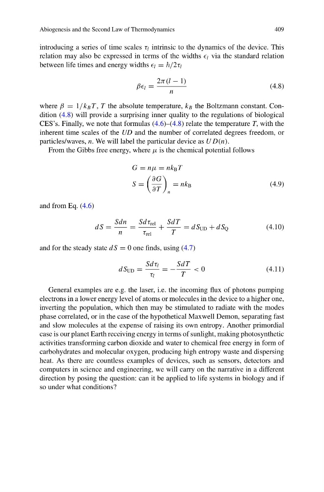
introducing a series of time scales τ l intrinsic to the dynamics of the device. This
relation may also be expressed in terms of the widths l via the standard relation
between life times and energy widths l = /2τ l
ββ l =
2π (l − 1)
n
(4.8)
where β = 1/k B T , T the absolute temperature, k B the Boltzmann constant. Condition (4.8) will provide a surprising inner quality to the regulations of biological
CES’s. Finally, we note that formulas (4.6)–(4.8) relate the temperature T, with the
inherent time scales of the UD and the number of correlated degrees freedom, or
particles/waves, n. We will label the particular device as U D(n).
From the Gibbs free energy, where μ is the chemical potential follows
G = nμ = nk B T
S =
∂G
∂ T
n
= nk B
(4.9)
and from Eq. (4.6)
d S =
Sdn
n
=
Sdτ rel
τ rel
+
SdT
T
= d S UD + d S Q
(4.10)
and for the steady state d S = 0 one finds, using (4.7)
d S UD =
Sdτ l
τ l
= −
SdT
T
< 0
(4.11)
General examples are e.g. the laser, i.e. the incoming flux of photons pumping
electrons in a lower energy level of atoms or molecules in the device to a higher one,
inverting the population, which then may be stimulated to radiate with the modes
phase correlated, or in the case of the hypothetical Maxwell Demon, separating fast
and slow molecules at the expense of raising its own entropy. Another primordial
case is our planet Earth receiving energy in terms of sunlight, making photosynthetic
activities transforming carbon dioxide and water to chemical free energy in form of
carbohydrates and molecular oxygen, producing high entropy waste and dispersing
heat. As there are countless examples of devices, such as sensors, detectors and
computers in science and engineering, we will carry on the narrative in a different
direction by posing the question: can it be applied to life systems in biology and if
so under what conditions?
409
introducing a series of time scales τ l intrinsic to the dynamics of the device. This
relation may also be expressed in terms of the widths l via the standard relation
between life times and energy widths l = /2τ l
ββ l =
2π (l − 1)
n
(4.8)
where β = 1/k B T , T the absolute temperature, k B the Boltzmann constant. Condition (4.8) will provide a surprising inner quality to the regulations of biological
CES’s. Finally, we note that formulas (4.6)–(4.8) relate the temperature T, with the
inherent time scales of the UD and the number of correlated degrees freedom, or
particles/waves, n. We will label the particular device as U D(n).
From the Gibbs free energy, where μ is the chemical potential follows
G = nμ = nk B T
S =
∂G
∂ T
n
= nk B
(4.9)
and from Eq. (4.6)
d S =
Sdn
n
=
Sdτ rel
τ rel
+
SdT
T
= d S UD + d S Q
(4.10)
and for the steady state d S = 0 one finds, using (4.7)
d S UD =
Sdτ l
τ l
= −
SdT
T
< 0
(4.11)
General examples are e.g. the laser, i.e. the incoming flux of photons pumping
electrons in a lower energy level of atoms or molecules in the device to a higher one,
inverting the population, which then may be stimulated to radiate with the modes
phase correlated, or in the case of the hypothetical Maxwell Demon, separating fast
and slow molecules at the expense of raising its own entropy. Another primordial
case is our planet Earth receiving energy in terms of sunlight, making photosynthetic
activities transforming carbon dioxide and water to chemical free energy in form of
carbohydrates and molecular oxygen, producing high entropy waste and dispersing
heat. As there are countless examples of devices, such as sensors, detectors and
computers in science and engineering, we will carry on the narrative in a different
direction by posing the question: can it be applied to life systems in biology and if
so under what conditions?