

Efficient “Middle” Thermostat Scheme …
275
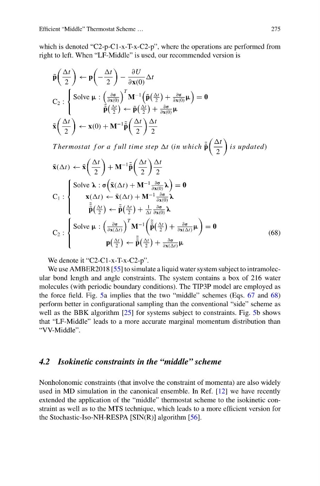
which is denoted “C2-p-C1-x-T-x-C2-p”, where the operations are performed from
right to left. When “LF-Middle” is used, our recommended version is
˜
p
t
2
← p
−
t
2
−
∂U
∂x(0)
t
C 2 :
⎧
⎨
⎩
Solve μ :
∂σ
∂x(0)
T
M
−1
˜
p
t
2
+
∂σ
∂x(0)
μ
= 0
˜ ˜
p
t
2
← ˜
p
t
2
+
∂σ
∂x(0)
μ
˜
x
t
2
← x(0) + M
−1 ˜ ˜
p
t
2
t
2
T hermostat f or a f ull time step t (in which ˜ ˜
p
t
2
is updated)
˜
x(t) ← ˜
x
t
2
+ M
−1 ˜ ˜
p
t
2
t
2
C 1 :
⎧
⎪ ⎪ ⎨
⎪ ⎪ ⎩
Solve λ : σ
˜
x(t) + M
−1 ∂σ
∂x(0)
λ
= 0
x(t) ← ˜
x(t) + M
−1 ∂σ
∂x(0)
λ
˜ ˜ ˜
p
t
2
← ˜ ˜
p
t
2
+
1
t
∂σ
∂x(0)
λ
C 2 :
⎧
⎪ ⎨
⎪ ⎩
Solve μ :
∂σ
∂x(t)
T
M
−1
˜ ˜ ˜
p
t
2
+
∂σ
∂x(t)
μ
= 0
p
t
2
←
˜ ˜ ˜
p
t
2
+
∂σ
∂x(t)
μ
(68)
We denote it “C2-C1-x-T-x-C2-p”.
We use AMBER2018 [55] to simulate a liquid water system subject to intramolecular bond length and angle constraints. The system contains a box of 216 water
molecules (with periodic boundary conditions). The TIP3P model are employed as
the force field. Fig. 5a implies that the two “middle” schemes (Eqs. 67 and 68)
perform better in configurational sampling than the conventional “side” scheme as
well as the BBK algorithm [25] for systems subject to constraints. Fig. 5b shows
that “LF-Middle” leads to a more accurate marginal momentum distribution than
“VV-Middle”.
4.2 Isokinetic constraints in the “middle” scheme
Nonholonomic constraints (that involve the constraint of momenta) are also widely
used in MD simulation in the canonical ensemble. In Ref. [12] we have recently
extended the application of the “middle” thermostat scheme to the isokinetic constraint as well as to the MTS technique, which leads to a more efficient version for
the Stochastic-Iso-NH-RESPA [SIN(R)] algorithm [56].
275
which is denoted “C2-p-C1-x-T-x-C2-p”, where the operations are performed from
right to left. When “LF-Middle” is used, our recommended version is
˜
p
t
2
← p
−
t
2
−
∂U
∂x(0)
t
C 2 :
⎧
⎨
⎩
Solve μ :
∂σ
∂x(0)
T
M
−1
˜
p
t
2
+
∂σ
∂x(0)
μ
= 0
˜ ˜
p
t
2
← ˜
p
t
2
+
∂σ
∂x(0)
μ
˜
x
t
2
← x(0) + M
−1 ˜ ˜
p
t
2
t
2
T hermostat f or a f ull time step t (in which ˜ ˜
p
t
2
is updated)
˜
x(t) ← ˜
x
t
2
+ M
−1 ˜ ˜
p
t
2
t
2
C 1 :
⎧
⎪ ⎪ ⎨
⎪ ⎪ ⎩
Solve λ : σ
˜
x(t) + M
−1 ∂σ
∂x(0)
λ
= 0
x(t) ← ˜
x(t) + M
−1 ∂σ
∂x(0)
λ
˜ ˜ ˜
p
t
2
← ˜ ˜
p
t
2
+
1
t
∂σ
∂x(0)
λ
C 2 :
⎧
⎪ ⎨
⎪ ⎩
Solve μ :
∂σ
∂x(t)
T
M
−1
˜ ˜ ˜
p
t
2
+
∂σ
∂x(t)
μ
= 0
p
t
2
←
˜ ˜ ˜
p
t
2
+
∂σ
∂x(t)
μ
(68)
We denote it “C2-C1-x-T-x-C2-p”.
We use AMBER2018 [55] to simulate a liquid water system subject to intramolecular bond length and angle constraints. The system contains a box of 216 water
molecules (with periodic boundary conditions). The TIP3P model are employed as
the force field. Fig. 5a implies that the two “middle” schemes (Eqs. 67 and 68)
perform better in configurational sampling than the conventional “side” scheme as
well as the BBK algorithm [25] for systems subject to constraints. Fig. 5b shows
that “LF-Middle” leads to a more accurate marginal momentum distribution than
“VV-Middle”.
4.2 Isokinetic constraints in the “middle” scheme
Nonholonomic constraints (that involve the constraint of momenta) are also widely
used in MD simulation in the canonical ensemble. In Ref. [12] we have recently
extended the application of the “middle” thermostat scheme to the isokinetic constraint as well as to the MTS technique, which leads to a more efficient version for
the Stochastic-Iso-NH-RESPA [SIN(R)] algorithm [56].