

274
X. Liu et al.
4 “Middle” scheme with constraints
4.1 Holonomic constraint
Define the holonomic constraint
σ(x) = 0,
(65)
where σ(x) is n c -dimensional vector function of the configuration x. Its derivative
yields the constraint for the momentum p
d
dt
σ(x) =
∂σ
∂x
T
M
−1 p = 0.
(66)
SHAKE [53] and RATTLE [54] are two typical algorithms for applying constraints to molecular systems. While SHAKE guarantees only the position constraint,
RATTLE satisfies both the position and momentum constraints. It is straightforward
to employ the “middle” scheme with the SHAKE or RATTLE algorithm for sampling
the canonical (NVT) ensemble. Various versions can be constructed to guarantee
that the position and momentum satisfy Eqs. (65)–(66) at the end of a time step. Our
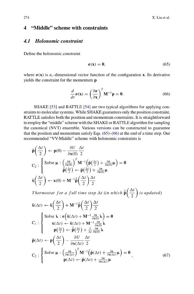
recommended “VV-Middle” scheme with holonomic constraints is
˜
p
t
2
← p(0) −
∂U
∂x(0)
t
2
C 2 :
⎧
⎨
⎩
Solve μ :
∂σ
∂x(0)
T
M
−1
˜
p
t
2
+
∂σ
∂x(0)
μ
= 0
˜ ˜
p
t
2
← ˜
p
t
2
+
∂σ
∂x(0)
μ
˜
x
t
2
← x(0) + M
−1 ˜ ˜
p
t
2
t
2
T hermostat f or a f ull time step t (in which ˜ ˜
p
t
2
is updated)
˜
x(t) ← ˜
x
t
2
+ M
−1 ˜ ˜
p
t
2
t
2
C 1 :
⎧
⎪ ⎪ ⎨
⎪ ⎪ ⎩
Solve λ : σ
˜
x(t) + M
−1 ∂σ
∂x(0)
λ
= 0
x(t) ← ˜
x(t) + M
−1 ∂σ
∂x(0)
λ
p
t
2
← ˜ ˜
p
t
2
+
1
t
∂σ
∂x(0)
λ
˜
p(t) ← p
t
2
−
∂U
∂x(t)
t
2
C 2 :
⎧
⎨
⎩
Solve μ :
∂σ
∂x(t)
T
M
−1
˜
p(t) +
∂σ
∂x(t)
μ
= 0
p(t) ← ˜
p(t) +
∂σ
∂x(t)
μ
,
(67)
X. Liu et al.
4 “Middle” scheme with constraints
4.1 Holonomic constraint
Define the holonomic constraint
σ(x) = 0,
(65)
where σ(x) is n c -dimensional vector function of the configuration x. Its derivative
yields the constraint for the momentum p
d
dt
σ(x) =
∂σ
∂x
T
M
−1 p = 0.
(66)
SHAKE [53] and RATTLE [54] are two typical algorithms for applying constraints to molecular systems. While SHAKE guarantees only the position constraint,
RATTLE satisfies both the position and momentum constraints. It is straightforward
to employ the “middle” scheme with the SHAKE or RATTLE algorithm for sampling
the canonical (NVT) ensemble. Various versions can be constructed to guarantee
that the position and momentum satisfy Eqs. (65)–(66) at the end of a time step. Our
recommended “VV-Middle” scheme with holonomic constraints is
˜
p
t
2
← p(0) −
∂U
∂x(0)
t
2
C 2 :
⎧
⎨
⎩
Solve μ :
∂σ
∂x(0)
T
M
−1
˜
p
t
2
+
∂σ
∂x(0)
μ
= 0
˜ ˜
p
t
2
← ˜
p
t
2
+
∂σ
∂x(0)
μ
˜
x
t
2
← x(0) + M
−1 ˜ ˜
p
t
2
t
2
T hermostat f or a f ull time step t (in which ˜ ˜
p
t
2
is updated)
˜
x(t) ← ˜
x
t
2
+ M
−1 ˜ ˜
p
t
2
t
2
C 1 :
⎧
⎪ ⎪ ⎨
⎪ ⎪ ⎩
Solve λ : σ
˜
x(t) + M
−1 ∂σ
∂x(0)
λ
= 0
x(t) ← ˜
x(t) + M
−1 ∂σ
∂x(0)
λ
p
t
2
← ˜ ˜
p
t
2
+
1
t
∂σ
∂x(0)
λ
˜
p(t) ← p
t
2
−
∂U
∂x(t)
t
2
C 2 :
⎧
⎨
⎩
Solve μ :
∂σ
∂x(t)
T
M
−1
˜
p(t) +
∂σ
∂x(t)
μ
= 0
p(t) ← ˜
p(t) +
∂σ
∂x(t)
μ
,
(67)