

Efficient “Middle” Thermostat Scheme …
273
Their coupling to a thermostat produces a proper canonical distribution for
(R 1 , . . . , R P ; p 1 , . . . , p P ), which changes Eq. (60) into
ˆ
B
= lim
P→∞
P
i=1
dR i dp i
exp
−β H
(dia)
eff (R 1 , . . . , R P ; p 1 , . . . , p P )
˜
B (dia) (R 1 , . . . , R P )
P
i=1
dR i dp i
exp
−β H
(dia)
eff (R 1 , . . . , R P ; p 1 , . . . , p P )
˜
Z (dia) (R 1 , . . . , R P )
. (63)
Similar to Eq. (37), the MES-PIMD equations of motion are decomposed into
three parts
˙
R i
˙
p i
=
˜
M
−1
i p i
0
x
+
0
−
∂U
(dia)
eff
∂R i
p
+ (Thermostat)
T
i = 1, P
.
(64)
The “middle” scheme then yields efficient MES-PIMD algorithms. As discussed
in Sects. 3.2 and 3.3, the staging or normal-mode transformation of path integral
beads can be used in Eq. (64).
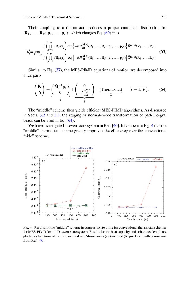
We have investigated a seven-state system in Ref. [40]. It is shown in Fig. 4 that the
“middle” thermostat scheme greatly improves the efficiency over the conventional
“side” scheme.
2 10
-6
3 10
-6
4 10
-6
5 10
-6
6 10
-6
7 10
-6
8 10
-6
9 10
-6
1 10
-5
0
100 200 300 400 500 600 700
1D-7state model
middle primitive
side primitive
middle virial
side virial
Heat
capacity C
V
(au/K)
Time interval Δt (au)
(c)
0.19
0.195
0.2
0.205
0.21
0.215
0.22
0
100 200 300 400 500 600 700
1D-7state model
middle
side
Coherence length L
coh
Time interval Δt (au)
(d)
Fig. 4 Results for the “middle” scheme in comparison to those for conventional thermostat schemes
for MES-PIMD for a 1-D seven-state system. Results for the heat capacity and coherence length are
plotted as functions of the time interval Atomic units (au) are used (Reproduced with permission
from Ref. [40])
273
Their coupling to a thermostat produces a proper canonical distribution for
(R 1 , . . . , R P ; p 1 , . . . , p P ), which changes Eq. (60) into
ˆ
B
= lim
P→∞
P
i=1
dR i dp i
exp
−β H
(dia)
eff (R 1 , . . . , R P ; p 1 , . . . , p P )
˜
B (dia) (R 1 , . . . , R P )
P
i=1
dR i dp i
exp
−β H
(dia)
eff (R 1 , . . . , R P ; p 1 , . . . , p P )
˜
Z (dia) (R 1 , . . . , R P )
. (63)
Similar to Eq. (37), the MES-PIMD equations of motion are decomposed into
three parts
˙
R i
˙
p i
=
˜
M
−1
i p i
0
x
+
0
−
∂U
(dia)
eff
∂R i
p
+ (Thermostat)
T
i = 1, P
.
(64)
The “middle” scheme then yields efficient MES-PIMD algorithms. As discussed
in Sects. 3.2 and 3.3, the staging or normal-mode transformation of path integral
beads can be used in Eq. (64).
We have investigated a seven-state system in Ref. [40]. It is shown in Fig. 4 that the
“middle” thermostat scheme greatly improves the efficiency over the conventional
“side” scheme.
2 10
-6
3 10
-6
4 10
-6
5 10
-6
6 10
-6
7 10
-6
8 10
-6
9 10
-6
1 10
-5
0
100 200 300 400 500 600 700
1D-7state model
middle primitive
side primitive
middle virial
side virial
Heat
capacity C
V
(au/K)
Time interval Δt (au)
(c)
0.19
0.195
0.2
0.205
0.21
0.215
0.22
0
100 200 300 400 500 600 700
1D-7state model
middle
side
Coherence length L
coh
Time interval Δt (au)
(d)
Fig. 4 Results for the “middle” scheme in comparison to those for conventional thermostat schemes
for MES-PIMD for a 1-D seven-state system. Results for the heat capacity and coherence length are
plotted as functions of the time interval Atomic units (au) are used (Reproduced with permission
from Ref. [40])