

276
X. Liu et al.
-2050
-2040
-2030
-2020
-2010
-2000
-1990
-1980
0
1
2
3
4
5
6
7
8
LF-Middle
VV-Middle
Side
Old
Potential energy (kcal/mol)
Time interval (fs)
(a)
355
360
365
370
375
380
385
390
395
0
1
2
3
4
5
6
7
8
Lf-Middle
VV-Middle
Side
Old
Kinetic energy (kcal/mol)
Time interval (fs)
(b)
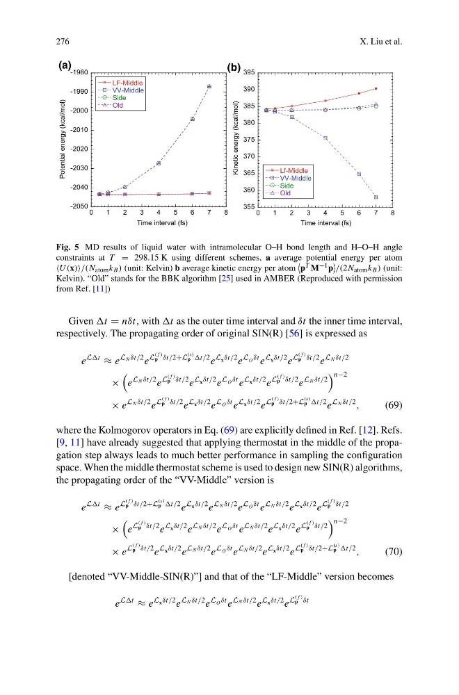
Fig. 5 MD results of liquid water with intramolecular O–H bond length and H–O–H angle
constraints at T = 298.15 K using different schemes, a average potential energy per atom
U (x)/(N atom k B ) (unit: Kelvin) b average kinetic energy per atom
p T M −1 p
/(2N atom k B ) (unit:
Kelvin). “Old” stands for the BBK algorithm [25] used in AMBER (Reproduced with permission
from Ref. [11])
Given = nδt, with as the outer time interval and δt the inner time interval,
respectively. The propagating order of original SIN(R) [56] is expressed as
e
L
≈ e
L N δt/2 e
L
( f )
p δt/2+L
(s)
p e
L x δt/2 e
L O δt e
L x δt/2 e
L
( f )
p δt/2 e
L N δt/2
×
e
L N δt/2 e
L
( f )
p δt/2 e
L x δt/2 e
L O δt e
L x δt/2 e
L
( f )
p δt/2 e
L N δt/2
n−2
× e
L N δt/2 e
L
( f )
p δt/2 e
L x δt/2 e
L O δt e
L x δt/2 e
L
( f )
p δt/2+L
(s)
p e
L N δt/2
,
(69)
where the Kolmogorov operators in Eq. (69) are explicitly defined in Ref. [12]. Refs.
[9, 11] have already suggested that applying thermostat in the middle of the propagation step always leads to much better performance in sampling the configuration
space. When the middle thermostat scheme is used to design new SIN(R) algorithms,
the propagating order of the “VV-Middle” version is
e
L
≈ e
L
( f )
p δt/2+L
(s)
p e
L x δt/2 e
L N δt/2 e
L O δt e
L N δt/2 e
L x δt/2 e
L
( f )
p δt/2
×
e
L
( f )
p δt/2 e
L x δt/2 e
L N δt/2 e
L O δt e
L N δt/2 e
L x δt/2 e
L
( f )
p δt/2
n−2
× e
L
( f )
p δt/2 e
L x δt/2 e
L N δt/2 e
L O δt e
L N δt/2 e
L x δt/2 e
L
( f )
p δt/2+L
(s)
p
,
(70)
[denoted “VV-Middle-SIN(R)”] and that of the “LF-Middle” version becomes
e
L
≈ e
L x δt/2 e
L N δt/2 e
L O δt e
L N δt/2 e
L x δt/2 e
L
( f )
p δt
X. Liu et al.
-2050
-2040
-2030
-2020
-2010
-2000
-1990
-1980
0
1
2
3
4
5
6
7
8
LF-Middle
VV-Middle
Side
Old
Potential energy (kcal/mol)
Time interval (fs)
(a)
355
360
365
370
375
380
385
390
395
0
1
2
3
4
5
6
7
8
Lf-Middle
VV-Middle
Side
Old
Kinetic energy (kcal/mol)
Time interval (fs)
(b)
Fig. 5 MD results of liquid water with intramolecular O–H bond length and H–O–H angle
constraints at T = 298.15 K using different schemes, a average potential energy per atom
U (x)/(N atom k B ) (unit: Kelvin) b average kinetic energy per atom
p T M −1 p
/(2N atom k B ) (unit:
Kelvin). “Old” stands for the BBK algorithm [25] used in AMBER (Reproduced with permission
from Ref. [11])
Given = nδt, with as the outer time interval and δt the inner time interval,
respectively. The propagating order of original SIN(R) [56] is expressed as
e
L
≈ e
L N δt/2 e
L
( f )
p δt/2+L
(s)
p e
L x δt/2 e
L O δt e
L x δt/2 e
L
( f )
p δt/2 e
L N δt/2
×
e
L N δt/2 e
L
( f )
p δt/2 e
L x δt/2 e
L O δt e
L x δt/2 e
L
( f )
p δt/2 e
L N δt/2
n−2
× e
L N δt/2 e
L
( f )
p δt/2 e
L x δt/2 e
L O δt e
L x δt/2 e
L
( f )
p δt/2+L
(s)
p e
L N δt/2
,
(69)
where the Kolmogorov operators in Eq. (69) are explicitly defined in Ref. [12]. Refs.
[9, 11] have already suggested that applying thermostat in the middle of the propagation step always leads to much better performance in sampling the configuration
space. When the middle thermostat scheme is used to design new SIN(R) algorithms,
the propagating order of the “VV-Middle” version is
e
L
≈ e
L
( f )
p δt/2+L
(s)
p e
L x δt/2 e
L N δt/2 e
L O δt e
L N δt/2 e
L x δt/2 e
L
( f )
p δt/2
×
e
L
( f )
p δt/2 e
L x δt/2 e
L N δt/2 e
L O δt e
L N δt/2 e
L x δt/2 e
L
( f )
p δt/2
n−2
× e
L
( f )
p δt/2 e
L x δt/2 e
L N δt/2 e
L O δt e
L N δt/2 e
L x δt/2 e
L
( f )
p δt/2+L
(s)
p
,
(70)
[denoted “VV-Middle-SIN(R)”] and that of the “LF-Middle” version becomes
e
L
≈ e
L x δt/2 e
L N δt/2 e
L O δt e
L N δt/2 e
L x δt/2 e
L
( f )
p δt