

Efficient “Middle” Thermostat Scheme …
259
Here, x and p are coordinates and momentum in vector forms, U (x) is the physical
potential energy, M the diagonal mass matrix.
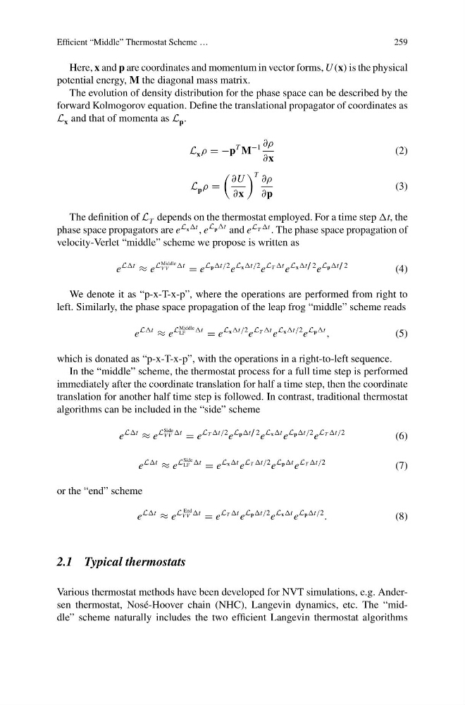
The evolution of density distribution for the phase space can be described by the
forward Kolmogorov equation. Define the translational propagator of coordinates as
L x and that of momenta as L p .
L x ρ = −p
T M
−1 ∂ρ
∂x
(2)
L p ρ =
∂U
∂x
T ∂ρ
∂p
(3)
The definition of L T depends on the thermostat employed. For a time step t, the
phase space propagators are e
L x t , e
L p t and e
L T t . The phase space propagation of
velocity-Verlet “middle” scheme we propose is written as
e
Lt
≈ e
L
Middle
V V
t
= e
L p t/2 e
L x t/2 e
L T t e
L x t / 2 e
L p t / 2
(4)
We denote it as “p-x-T-x-p”, where the operations are performed from right to
left. Similarly, the phase space propagation of the leap frog “middle” scheme reads
e
Lt
≈ e
L
Middle
LF
t
= e
L x t/2 e
L T t e
L x t/2 e
L p t
,
(5)
which is donated as “p-x-T-x-p”, with the operations in a right-to-left sequence.
In the “middle” scheme, the thermostat process for a full time step is performed
immediately after the coordinate translation for half a time step, then the coordinate
translation for another half time step is followed. In contrast, traditional thermostat
algorithms can be included in the “side” scheme
e
Lt
≈ e
L
Side
V V t
= e
L T t/2 e
L p t / 2 e
L x t e
L p t/2 e
L T t/2
(6)
e
Lt
≈ e
L
Side
LF t
= e
L x t e
L T t/2 e
L p t e
L T t/2
(7)
or the “end” scheme
e
Lt
≈ e
L
End
V V t
= e
L T t e
L p t/2 e
L x t e
L p t/2
.
(8)
2.1 Typical thermostats
Various thermostat methods have been developed for NVT simulations, e.g. Andersen thermostat, Nosé-Hoover chain (NHC), Langevin dynamics, etc. The “middle” scheme naturally includes the two efficient Langevin thermostat algorithms
259
Here, x and p are coordinates and momentum in vector forms, U (x) is the physical
potential energy, M the diagonal mass matrix.
The evolution of density distribution for the phase space can be described by the
forward Kolmogorov equation. Define the translational propagator of coordinates as
L x and that of momenta as L p .
L x ρ = −p
T M
−1 ∂ρ
∂x
(2)
L p ρ =
∂U
∂x
T ∂ρ
∂p
(3)
The definition of L T depends on the thermostat employed. For a time step t, the
phase space propagators are e
L x t , e
L p t and e
L T t . The phase space propagation of
velocity-Verlet “middle” scheme we propose is written as
e
Lt
≈ e
L
Middle
V V
t
= e
L p t/2 e
L x t/2 e
L T t e
L x t / 2 e
L p t / 2
(4)
We denote it as “p-x-T-x-p”, where the operations are performed from right to
left. Similarly, the phase space propagation of the leap frog “middle” scheme reads
e
Lt
≈ e
L
Middle
LF
t
= e
L x t/2 e
L T t e
L x t/2 e
L p t
,
(5)
which is donated as “p-x-T-x-p”, with the operations in a right-to-left sequence.
In the “middle” scheme, the thermostat process for a full time step is performed
immediately after the coordinate translation for half a time step, then the coordinate
translation for another half time step is followed. In contrast, traditional thermostat
algorithms can be included in the “side” scheme
e
Lt
≈ e
L
Side
V V t
= e
L T t/2 e
L p t / 2 e
L x t e
L p t/2 e
L T t/2
(6)
e
Lt
≈ e
L
Side
LF t
= e
L x t e
L T t/2 e
L p t e
L T t/2
(7)
or the “end” scheme
e
Lt
≈ e
L
End
V V t
= e
L T t e
L p t/2 e
L x t e
L p t/2
.
(8)
2.1 Typical thermostats
Various thermostat methods have been developed for NVT simulations, e.g. Andersen thermostat, Nosé-Hoover chain (NHC), Langevin dynamics, etc. The “middle” scheme naturally includes the two efficient Langevin thermostat algorithms