

260
X. Liu et al.
developed for MD in Refs. [29, 30, 32] and in Ref. [28] as shown in Ref. [15].
Below we briefly review the “middle” scheme with the Andersen thermostat and
Nosé-Hoover chain.
2.1.1 “Middle” scheme with the Andersen thermostat
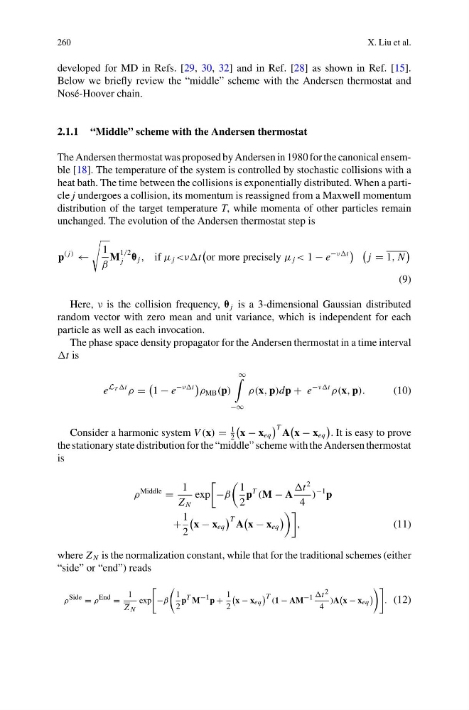
The Andersen thermostat was proposed by Andersen in 1980 for the canonical ensemble [18]. The temperature of the system is controlled by stochastic collisions with a
heat bath. The time between the collisions is exponentially distributed. When a particle j undergoes a collision, its momentum is reassigned from a Maxwell momentum
distribution of the target temperature T, while momenta of other particles remain
unchanged. The evolution of the Andersen thermostat step is
p
( j)
←
1
β
M
1/2
j θ j , if μ j <ννt
or more precisely μ j < 1 − e
−ννt
j = 1, N
(9)
Here, ν is the collision frequency, θ j is a 3-dimensional Gaussian distributed
random vector with zero mean and unit variance, which is independent for each
particle as well as each invocation.
The phase space density propagator for the Andersen thermostat in a time interval
t is
e
L T t
ρ =
1 − e
−ννt
ρ MB (p)
∞
−∞
ρ(x, p)dp + e
−ννt
ρ(x, p).
(10)
Consider a harmonic system V (x) =
1
2
x − x eq
T A
x − x eq
. It is easy to prove
the stationary state distribution for the “middle” scheme with the Andersen thermostat
is
ρ
Middle
=
1
Z N
exp
−β
1
2
p
T
(M − A
t
2
4
)
−1 p
+
1
2
x − x eq
T A
x − x eq
,
(11)
where Z N is the normalization constant, while that for the traditional schemes (either
“side” or “end”) reads
ρ Side = ρ End =
1
Z N
exp
−β
1
2
p T M −1 p +
1
2
x − x eq
T (1 − AM −1 t 2
4
)A
x − x eq
. (12)
X. Liu et al.
developed for MD in Refs. [29, 30, 32] and in Ref. [28] as shown in Ref. [15].
Below we briefly review the “middle” scheme with the Andersen thermostat and
Nosé-Hoover chain.
2.1.1 “Middle” scheme with the Andersen thermostat
The Andersen thermostat was proposed by Andersen in 1980 for the canonical ensemble [18]. The temperature of the system is controlled by stochastic collisions with a
heat bath. The time between the collisions is exponentially distributed. When a particle j undergoes a collision, its momentum is reassigned from a Maxwell momentum
distribution of the target temperature T, while momenta of other particles remain
unchanged. The evolution of the Andersen thermostat step is
p
( j)
←
1
β
M
1/2
j θ j , if μ j <ννt
or more precisely μ j < 1 − e
−ννt
j = 1, N
(9)
Here, ν is the collision frequency, θ j is a 3-dimensional Gaussian distributed
random vector with zero mean and unit variance, which is independent for each
particle as well as each invocation.
The phase space density propagator for the Andersen thermostat in a time interval
t is
e
L T t
ρ =
1 − e
−ννt
ρ MB (p)
∞
−∞
ρ(x, p)dp + e
−ννt
ρ(x, p).
(10)
Consider a harmonic system V (x) =
1
2
x − x eq
T A
x − x eq
. It is easy to prove
the stationary state distribution for the “middle” scheme with the Andersen thermostat
is
ρ
Middle
=
1
Z N
exp
−β
1
2
p
T
(M − A
t
2
4
)
−1 p
+
1
2
x − x eq
T A
x − x eq
,
(11)
where Z N is the normalization constant, while that for the traditional schemes (either
“side” or “end”) reads
ρ Side = ρ End =
1
Z N
exp
−β
1
2
p T M −1 p +
1
2
x − x eq
T (1 − AM −1 t 2
4
)A
x − x eq
. (12)