

258
X. Liu et al.
In this review we focus on recent progress on the efficient “middle” thermostat
[9–12] that has been established in a series of papers [7, 9, 11–16] and has been implemented in AMBER [17] (the 2018 and 2019 versions). In 2016 we first suggested the
Langevin thermostat in the “middle” scheme to construct efficient sampling algorithms for PIMD [7, 13, 14]. In 2017 and 2018 we developed a unified framework
[9, 11] based on either velocity-Verlet or leap-frog algorithms to apply various thermostat algorithms for MD [1, 15, 18–32] and those for PIMD [7, 13, 14, 33–39]
proposed for the canonical (NVT) ensemble. In our unified theoretical framework,
we can describe most conventional algorithms [1, 15, 18–27, 33–36, 38, 39] in the
“side” or “end” scheme. The unified “middle” scheme we proposed in Refs. [9, 11]
provides an efficient tool for configurational sampling with either stochastic or deterministic thermostats. We have further extended the “middle” thermostat scheme as
an efficient configurational sampling tool for systems with holonomic or isokinetic
constraints [12]. Even when multiple-time-step (MTS) techniques are employed, the
“middle” scheme leads to new algorithms that outperform original ones [12]. We
have recently extended PIMD to offer an exact tool for quantum statistical properties in coupled multi-electronic-state systems [40, 41] where the Born-Oppenheimer
approximation breaks down, in which the “middle” thermostat scheme still offers an
efficient sampling tool.
2 “Middle” scheme
The “middle” scheme for MD or PIMD allows for larger time intervals to obtain the
same convergence value, which significantly reduces the computational cost. The
“middle” scheme is a powerful tool for configurational sampling, thus is helpful for
evaluating thermodynamic properties that depend on coordinates in classical MD
simulation For PIMD, all the structural and thermodynamic properties in quantum
mechanics are functions of only the configurations of the path integral beads, the
“middle” scheme is particularly useful because the time interval can be increased by
4 to 10 times without loss of accuracy.
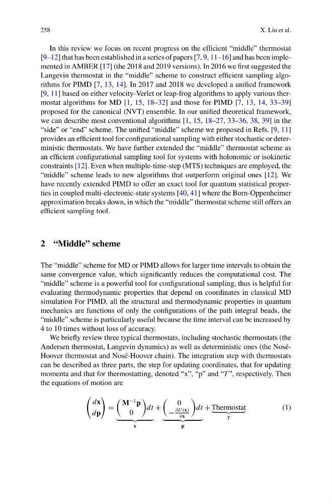
We briefly review three typical thermostats, including stochastic thermostats (the
Andersen thermostat, Langevin dynamics) as well as deterministic ones (the NoséHoover thermostat and Nosé-Hoover chain). The integration step with thermostats
can be described as three parts, the step for updating coordinates, that for updating
momenta and that for thermostatting, denoted “x”, “p” and “T ”, respectively. Then
the equations of motion are
dx
dp
=
M
−1 p
0
dt
x
+
0
−
∂U (x)
∂x
dt
p
+ Thermostat
T
(1)
X. Liu et al.
In this review we focus on recent progress on the efficient “middle” thermostat
[9–12] that has been established in a series of papers [7, 9, 11–16] and has been implemented in AMBER [17] (the 2018 and 2019 versions). In 2016 we first suggested the
Langevin thermostat in the “middle” scheme to construct efficient sampling algorithms for PIMD [7, 13, 14]. In 2017 and 2018 we developed a unified framework
[9, 11] based on either velocity-Verlet or leap-frog algorithms to apply various thermostat algorithms for MD [1, 15, 18–32] and those for PIMD [7, 13, 14, 33–39]
proposed for the canonical (NVT) ensemble. In our unified theoretical framework,
we can describe most conventional algorithms [1, 15, 18–27, 33–36, 38, 39] in the
“side” or “end” scheme. The unified “middle” scheme we proposed in Refs. [9, 11]
provides an efficient tool for configurational sampling with either stochastic or deterministic thermostats. We have further extended the “middle” thermostat scheme as
an efficient configurational sampling tool for systems with holonomic or isokinetic
constraints [12]. Even when multiple-time-step (MTS) techniques are employed, the
“middle” scheme leads to new algorithms that outperform original ones [12]. We
have recently extended PIMD to offer an exact tool for quantum statistical properties in coupled multi-electronic-state systems [40, 41] where the Born-Oppenheimer
approximation breaks down, in which the “middle” thermostat scheme still offers an
efficient sampling tool.
2 “Middle” scheme
The “middle” scheme for MD or PIMD allows for larger time intervals to obtain the
same convergence value, which significantly reduces the computational cost. The
“middle” scheme is a powerful tool for configurational sampling, thus is helpful for
evaluating thermodynamic properties that depend on coordinates in classical MD
simulation For PIMD, all the structural and thermodynamic properties in quantum
mechanics are functions of only the configurations of the path integral beads, the
“middle” scheme is particularly useful because the time interval can be increased by
4 to 10 times without loss of accuracy.
We briefly review three typical thermostats, including stochastic thermostats (the
Andersen thermostat, Langevin dynamics) as well as deterministic ones (the NoséHoover thermostat and Nosé-Hoover chain). The integration step with thermostats
can be described as three parts, the step for updating coordinates, that for updating
momenta and that for thermostatting, denoted “x”, “p” and “T ”, respectively. Then
the equations of motion are
dx
dp
=
M
−1 p
0
dt
x
+
0
−
∂U (x)
∂x
dt
p
+ Thermostat
T
(1)