

Quantum Study of Helium Clusters Doped with Electronically Excited …
95
geometry implies an overlap of the two distributions (r HeHe =
1
2
r Ak H e ). As expected
from the potential energy surface study, the maximum of ρ Ak H e shifts towards larger
r i Ak values going from Li to Rb. At the same time the width of peak increases. For
Rb, the ρ HeHe is strictly overlapping the ρ Ak H e which is coherent with a linear HeRb
-He system as previously shown [51]. From Li to K, the comparison of ρ Ak H e
and ρ HeHe indicates that both linear and bent geometries are present. Moreover, the
ρ HeHe broadens as we go from Li to K which implies more floppy K
He 2 systems.
All of this is coherent with the double well picture I discussed in Sec. II. For Li, Na
and K, the wave function has thus no negligeable amplitudes in both the local and
global minima while for Rb
He 2 , the local bent minimum is too high in energy. The
angular distribution (not shown) confirms a mostly linear configuration for Rb and
a wide range from π /4 to π non-zero probability for
He Ak He angle for Li, Na and
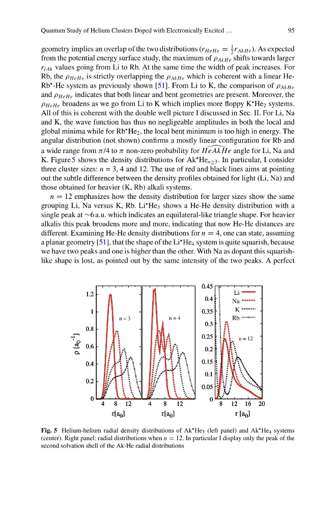
K. Figure 5 shows the density distributions for Ak
He n≥3 . In particular, I consider
three cluster sizes: n = 3, 4 and 12. The use of red and black lines aims at pointing
out the subtle difference between the density profiles obtained for light (Li, Na) and
those obtained for heavier (K, Rb) alkali systems.
n = 12 emphasizes how the density distribution for larger sizes show the same
grouping Li, Na versus K, Rb. Li
He 3 shows a He-He density distribution with a
single peak at ∼6 a.u. which indicates an equilateral-like triangle shape. For heavier
alkalis this peak broadens more and more, indicating that now He-He distances are
different. Examining He-He density distributions for n = 4, one can state, assuming
a planar geometry [51], that the shape of the Li
He 4 system is quite squarish, because
we have two peaks and one is higher than the other. With Na as dopant this squarishlike shape is lost, as pointed out by the same intensity of the two peaks. A perfect
0
0.2
0.4
0.6
0.8
1
1.2
4
8 12
ρ [a
0
-1
]
r[a 0 ]
0
0.2
0.4
0.6
0.8
1
1.2
4
8 12
ρ [a
0
-1
]
r[a 0 ]
0
0.2
0.4
0.6
0.8
1
1.2
4
8 12
ρ [a
0
-1
]
r[a 0 ]
0
0.2
0.4
0.6
0.8
1
1.2
4
8 12
ρ [a
0
-1
]
r[a 0 ]
n = 3
4
8
12
r[a 0 ]
4
8
12
r[a 0 ]
4
8
12
r[a 0 ]
4
8
12
r[a 0 ]
n = 4
0
0.05
0.1
0.15
0.2
0.25
0.3
0.35
0.4
0.45
8 12 16 20
r [a 0 ]
0
0.05
0.1
0.15
0.2
0.25
0.3
0.35
0.4
0.45
8 12 16 20
r [a 0 ]
0
0.05
0.1
0.15
0.2
0.25
0.3
0.35
0.4
0.45
8 12 16 20
r [a 0 ]
0
0.05
0.1
0.15
0.2
0.25
0.3
0.35
0.4
0.45
8 12 16 20
r [a 0 ]
n = 12
Li
Na
K
Rb
Fig. 5 Helium-helium radial density distributions of Ak He 3 (left panel) and Ak He 4 systems
(center). Right panel: radial distributions when n = 12. In particular I display only the peak of the
second solvation shell of the Ak-He radial distributions
95
geometry implies an overlap of the two distributions (r HeHe =
1
2
r Ak H e ). As expected
from the potential energy surface study, the maximum of ρ Ak H e shifts towards larger
r i Ak values going from Li to Rb. At the same time the width of peak increases. For
Rb, the ρ HeHe is strictly overlapping the ρ Ak H e which is coherent with a linear HeRb
-He system as previously shown [51]. From Li to K, the comparison of ρ Ak H e
and ρ HeHe indicates that both linear and bent geometries are present. Moreover, the
ρ HeHe broadens as we go from Li to K which implies more floppy K
He 2 systems.
All of this is coherent with the double well picture I discussed in Sec. II. For Li, Na
and K, the wave function has thus no negligeable amplitudes in both the local and
global minima while for Rb
He 2 , the local bent minimum is too high in energy. The
angular distribution (not shown) confirms a mostly linear configuration for Rb and
a wide range from π /4 to π non-zero probability for
He Ak He angle for Li, Na and
K. Figure 5 shows the density distributions for Ak
He n≥3 . In particular, I consider
three cluster sizes: n = 3, 4 and 12. The use of red and black lines aims at pointing
out the subtle difference between the density profiles obtained for light (Li, Na) and
those obtained for heavier (K, Rb) alkali systems.
n = 12 emphasizes how the density distribution for larger sizes show the same
grouping Li, Na versus K, Rb. Li
He 3 shows a He-He density distribution with a
single peak at ∼6 a.u. which indicates an equilateral-like triangle shape. For heavier
alkalis this peak broadens more and more, indicating that now He-He distances are
different. Examining He-He density distributions for n = 4, one can state, assuming
a planar geometry [51], that the shape of the Li
He 4 system is quite squarish, because
we have two peaks and one is higher than the other. With Na as dopant this squarishlike shape is lost, as pointed out by the same intensity of the two peaks. A perfect
0
0.2
0.4
0.6
0.8
1
1.2
4
8 12
ρ [a
0
-1
]
r[a 0 ]
0
0.2
0.4
0.6
0.8
1
1.2
4
8 12
ρ [a
0
-1
]
r[a 0 ]
0
0.2
0.4
0.6
0.8
1
1.2
4
8 12
ρ [a
0
-1
]
r[a 0 ]
0
0.2
0.4
0.6
0.8
1
1.2
4
8 12
ρ [a
0
-1
]
r[a 0 ]
n = 3
4
8
12
r[a 0 ]
4
8
12
r[a 0 ]
4
8
12
r[a 0 ]
4
8
12
r[a 0 ]
n = 4
0
0.05
0.1
0.15
0.2
0.25
0.3
0.35
0.4
0.45
8 12 16 20
r [a 0 ]
0
0.05
0.1
0.15
0.2
0.25
0.3
0.35
0.4
0.45
8 12 16 20
r [a 0 ]
0
0.05
0.1
0.15
0.2
0.25
0.3
0.35
0.4
0.45
8 12 16 20
r [a 0 ]
0
0.05
0.1
0.15
0.2
0.25
0.3
0.35
0.4
0.45
8 12 16 20
r [a 0 ]
n = 12
Li
Na
K
Rb
Fig. 5 Helium-helium radial density distributions of Ak He 3 (left panel) and Ak He 4 systems
(center). Right panel: radial distributions when n = 12. In particular I display only the peak of the
second solvation shell of the Ak-He radial distributions