

94
D. Dell’Angelo
atoms [56]. In the first shell systematic increase of the chemical potential is obtained
for Li and Na when n increases from 2 to 5. For K and Rb, the energy gained adding
the fourth He atom is greater than the one for adding the third one. The relative
energy difference between the two last He atoms which fill the first shell decreases
moving down the alkali series: we can infer that the escape probability of one He
atom from the filled shell decreases in the same way. For larger n, He atoms are much
more weakly bound. A second drop in the absolute value of the chemical potential
can suggest the closing of the second shell. Anyway, this drop is less pronounced
for Li and Na. Thus at this level one can observe that a closure of the second shell
possibly corresponds to 9 atoms for Li, 10 for Na, 11 for K and Rb. Yet, if we look
at the μ(n) of Li, we may also suppose a closure to 10 atoms: density distributions
introduced below will add structural informations to better analyze this issue. With
the small number of helium atoms considered in this work, the chemical potential
values are still far from the pure cluster limit.
3.3 Densities
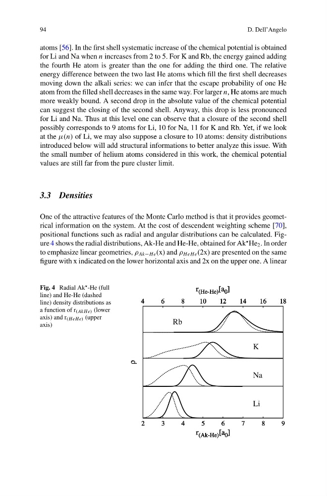
One of the attractive features of the Monte Carlo method is that it provides geometrical information on the system. At the cost of descendent weighting scheme [70],
positional functions such as radial and angular distributions can be calculated. Figure 4 shows the radial distributions, Ak-He and He-He, obtained for Ak
He 2 . In order
to emphasize linear geometries, ρ Ak−He (x) and ρ HeHe (2x) are presented on the same
figure with x indicated on the lower horizontal axis and 2x on the upper one. A linear
Fig. 4 Radial Ak -He (full
line) and He-He (dashed
line) density distributions as
a function of r (Ak H e) (lower
axis) and r (HeHe) (upper
axis)
2
3
4
5
6
7
8
9
4
6
8
10
12
14
16
18
ρ
r (Ak-He) [a 0 ]
r (He-He) [a 0 ]
2
3
4
5
6
7
8
9
4
6
8
10
12
14
16
18
ρ
r (Ak-He) [a 0 ]
r (He-He) [a 0 ]
2
3
4
5
6
7
8
9
4
6
8
10
12
14
16
18
ρ
r (Ak-He) [a 0 ]
r (He-He) [a 0 ]
2
3
4
5
6
7
8
9
4
6
8
10
12
14
16
18
ρ
r (Ak-He) [a 0 ]
r (He-He) [a 0 ]
2
3
4
5
6
7
8
9
4
6
8
10
12
14
16
18
ρ
r (Ak-He) [a 0 ]
r (He-He) [a 0 ]
2
3
4
5
6
7
8
9
4
6
8
10
12
14
16
18
ρ
r (Ak-He) [a 0 ]
r (He-He) [a 0 ]
2
3
4
5
6
7
8
9
4
6
8
10
12
14
16
18
ρ
r (Ak-He) [a 0 ]
r (He-He) [a 0 ]
Li
Na
K
Rb
D. Dell’Angelo
atoms [56]. In the first shell systematic increase of the chemical potential is obtained
for Li and Na when n increases from 2 to 5. For K and Rb, the energy gained adding
the fourth He atom is greater than the one for adding the third one. The relative
energy difference between the two last He atoms which fill the first shell decreases
moving down the alkali series: we can infer that the escape probability of one He
atom from the filled shell decreases in the same way. For larger n, He atoms are much
more weakly bound. A second drop in the absolute value of the chemical potential
can suggest the closing of the second shell. Anyway, this drop is less pronounced
for Li and Na. Thus at this level one can observe that a closure of the second shell
possibly corresponds to 9 atoms for Li, 10 for Na, 11 for K and Rb. Yet, if we look
at the μ(n) of Li, we may also suppose a closure to 10 atoms: density distributions
introduced below will add structural informations to better analyze this issue. With
the small number of helium atoms considered in this work, the chemical potential
values are still far from the pure cluster limit.
3.3 Densities
One of the attractive features of the Monte Carlo method is that it provides geometrical information on the system. At the cost of descendent weighting scheme [70],
positional functions such as radial and angular distributions can be calculated. Figure 4 shows the radial distributions, Ak-He and He-He, obtained for Ak
He 2 . In order
to emphasize linear geometries, ρ Ak−He (x) and ρ HeHe (2x) are presented on the same
figure with x indicated on the lower horizontal axis and 2x on the upper one. A linear
Fig. 4 Radial Ak -He (full
line) and He-He (dashed
line) density distributions as
a function of r (Ak H e) (lower
axis) and r (HeHe) (upper
axis)
2
3
4
5
6
7
8
9
4
6
8
10
12
14
16
18
ρ
r (Ak-He) [a 0 ]
r (He-He) [a 0 ]
2
3
4
5
6
7
8
9
4
6
8
10
12
14
16
18
ρ
r (Ak-He) [a 0 ]
r (He-He) [a 0 ]
2
3
4
5
6
7
8
9
4
6
8
10
12
14
16
18
ρ
r (Ak-He) [a 0 ]
r (He-He) [a 0 ]
2
3
4
5
6
7
8
9
4
6
8
10
12
14
16
18
ρ
r (Ak-He) [a 0 ]
r (He-He) [a 0 ]
2
3
4
5
6
7
8
9
4
6
8
10
12
14
16
18
ρ
r (Ak-He) [a 0 ]
r (He-He) [a 0 ]
2
3
4
5
6
7
8
9
4
6
8
10
12
14
16
18
ρ
r (Ak-He) [a 0 ]
r (He-He) [a 0 ]
2
3
4
5
6
7
8
9
4
6
8
10
12
14
16
18
ρ
r (Ak-He) [a 0 ]
r (He-He) [a 0 ]
Li
Na
K
Rb