

Basics of beam dynamics 9
(a)
Dipole
(b)
Quadrupole
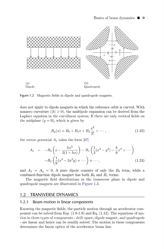
Figure 1.2 Magnetic fields in dipole and quadrupole magnets.
does not apply to dipole magnets in which the reference orbit is curved. With
nonzero curvature (|h| > 0), the multipole expansion can be derived from the
Laplace equation in the curvilinear system. If there are only vertical fields on
the midplane (y = 0), which is given by
B y (x) = B 0 + B 1 x + B 2
x
2
2!
+ · · · ,
(1.22)
the vector potential A s takes the form [67]
A s = −B 0
x −
hx
2
2(1 + hx)
− B 1
1
2
(x
2 − y
2 ) −
h
6
x
3 + · · ·
−B 2
1
6
(x
3 − 3x
2 y) + · · ·
+ · · · ,
(1.23)
and A x = A y = 0. A pure dipole consists of only the B 0 term, while a
combined-function dipole magnet has both B 0 and B 1 terms.
The magnetic field distributions in the transverse plane in dipole and
quadrupole magnets are illustrated in Figure 1.2.
1.2 TRANSVERSE DYNAMICS
1.2.1 Beam motion in linear components
Knowing the magnetic fields, the particle motion through an accelerator component can be solved from Eqs. (1.8-1.9) and Eq. (1.12). The equations of motion in three types of components - drift space, dipole magnet, and quadrupole
- are linear and hence can be readily solved. The motion in these components
determines the linear optics of the accelerator beam line.
(a)
Dipole
(b)
Quadrupole
Figure 1.2 Magnetic fields in dipole and quadrupole magnets.
does not apply to dipole magnets in which the reference orbit is curved. With
nonzero curvature (|h| > 0), the multipole expansion can be derived from the
Laplace equation in the curvilinear system. If there are only vertical fields on
the midplane (y = 0), which is given by
B y (x) = B 0 + B 1 x + B 2
x
2
2!
+ · · · ,
(1.22)
the vector potential A s takes the form [67]
A s = −B 0
x −
hx
2
2(1 + hx)
− B 1
1
2
(x
2 − y
2 ) −
h
6
x
3 + · · ·
−B 2
1
6
(x
3 − 3x
2 y) + · · ·
+ · · · ,
(1.23)
and A x = A y = 0. A pure dipole consists of only the B 0 term, while a
combined-function dipole magnet has both B 0 and B 1 terms.
The magnetic field distributions in the transverse plane in dipole and
quadrupole magnets are illustrated in Figure 1.2.
1.2 TRANSVERSE DYNAMICS
1.2.1 Beam motion in linear components
Knowing the magnetic fields, the particle motion through an accelerator component can be solved from Eqs. (1.8-1.9) and Eq. (1.12). The equations of motion in three types of components - drift space, dipole magnet, and quadrupole
- are linear and hence can be readily solved. The motion in these components
determines the linear optics of the accelerator beam line.