

Online optimization algorithms 199
0
50
100
150
200
250
300
evaluations
10
-4
10
-2
10
0
y = f(x)
RCDS, N=300
=0.001
=0.01
=0.1
0
20
40
60
80
100
cases
10
-4
10
-2
10
0
f
min
RCDS, N=300
=0.001
=0.01
=0.1
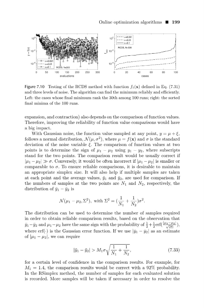
Figure 7.10 Testing of the RCDS method with function f1(x) defined in Eq. (7.31)
and three levels of noise. The algorithm can find the minimum reliably and efficiently.
Left: the cases whose final minimum rank the 30th among 100 runs; right: the sorted
final minima of the 100 runs.
expansion, and contraction) also depends on the comparison of function values.
Therefore, improving the reliability of function value comparisons would have
a big impact.
With Gaussian noise, the function value sampled at any point, y = µ + ξ,
follows a normal distribution, N (µ, σ
2 ), where µ = f (x) and σ is the standard
deviation of the noise variable ξ. The comparison of function values at two
points is to determine the sign of µ 1 − µ 2 using y 1 − y 2 , where subscripts
stand for the two points. The comparison result would be usually correct if
|µ 1 − µ 2 | | σ. Conversely, it would be often incorrect if |µ 1 − µ 2 | is smaller or
comparable to σ. To ensure reliable comparisons, it is desirable to maintain
an appropriate simplex size. It will also help if multiple samples are taken
at each point and the average values, ¯
y 1 and ¯
y 2 , are used for comparison. If
the numbers of samples at the two points are N 1 and N 2 , respectively, the
distribution of ¯
y 1 − ¯
y 2 is
N (µ 1 − µ 2 , Σ
2 ), with Σ
2 = (
1
N 1
+
1
N 2
)σ
2 .
The distribution can be used to determine the number of samples required
in order to obtain reliable comparison results, based on the observation that
¯
y 1 − ¯
y 2 and µ 1 −µ 2 have the same sign with the probability of
1
2 +
1
2 erf(
|µ1−µ2|
√
2Σ
),
where erf(·) is the Gaussian error function. If we use |¯ y 1 − ¯
y 2 | as an estimate
of |µ 1 − µ 2 |, we can require
|¯ y 1 − ¯
y 2 | > M 1 σ
1
N 1
+
1
N 2
,
(7.33)
for a certain level of confidence in the comparison results. For example, for
M 1 = 1.4, the comparison results would be correct with a 92% probability.
In the RSimplex method, the number of samples for each evaluated solution
is recorded. More samples will be taken if necessary in order to resolve the
0
50
100
150
200
250
300
evaluations
10
-4
10
-2
10
0
y = f(x)
RCDS, N=300
=0.001
=0.01
=0.1
0
20
40
60
80
100
cases
10
-4
10
-2
10
0
f
min
RCDS, N=300
=0.001
=0.01
=0.1
Figure 7.10 Testing of the RCDS method with function f1(x) defined in Eq. (7.31)
and three levels of noise. The algorithm can find the minimum reliably and efficiently.
Left: the cases whose final minimum rank the 30th among 100 runs; right: the sorted
final minima of the 100 runs.
expansion, and contraction) also depends on the comparison of function values.
Therefore, improving the reliability of function value comparisons would have
a big impact.
With Gaussian noise, the function value sampled at any point, y = µ + ξ,
follows a normal distribution, N (µ, σ
2 ), where µ = f (x) and σ is the standard
deviation of the noise variable ξ. The comparison of function values at two
points is to determine the sign of µ 1 − µ 2 using y 1 − y 2 , where subscripts
stand for the two points. The comparison result would be usually correct if
|µ 1 − µ 2 | | σ. Conversely, it would be often incorrect if |µ 1 − µ 2 | is smaller or
comparable to σ. To ensure reliable comparisons, it is desirable to maintain
an appropriate simplex size. It will also help if multiple samples are taken
at each point and the average values, ¯
y 1 and ¯
y 2 , are used for comparison. If
the numbers of samples at the two points are N 1 and N 2 , respectively, the
distribution of ¯
y 1 − ¯
y 2 is
N (µ 1 − µ 2 , Σ
2 ), with Σ
2 = (
1
N 1
+
1
N 2
)σ
2 .
The distribution can be used to determine the number of samples required
in order to obtain reliable comparison results, based on the observation that
¯
y 1 − ¯
y 2 and µ 1 −µ 2 have the same sign with the probability of
1
2 +
1
2 erf(
|µ1−µ2|
√
2Σ
),
where erf(·) is the Gaussian error function. If we use |¯ y 1 − ¯
y 2 | as an estimate
of |µ 1 − µ 2 |, we can require
|¯ y 1 − ¯
y 2 | > M 1 σ
1
N 1
+
1
N 2
,
(7.33)
for a certain level of confidence in the comparison results. For example, for
M 1 = 1.4, the comparison results would be correct with a 92% probability.
In the RSimplex method, the number of samples for each evaluated solution
is recorded. More samples will be taken if necessary in order to resolve the