

194 Beam-based Correction and Optimization for Accelerators
0
50
100
150
200
250
300
evaluations
10
-4
10
-2
10
0
y = f(x)
GD, N=300
=0.001
=0.01
=0.1
0
20
40
60
80
100
cases
10
-4
10
-2
10
0
f
min
GD, N=300
=0.001
=0.01
=0.1
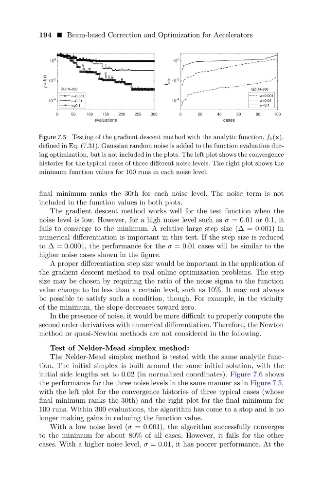
Figure 7.5 Testing of the gradient descent method with the analytic function, f1(x),
defined in Eq. (7.31). Gaussian random noise is added to the function evaluation during optimization, but is not included in the plots. The left plot shows the convergence
histories for the typical cases of three different noise levels. The right plot shows the
minimum function values for 100 runs in each noise level.
final minimum ranks the 30th for each noise level. The noise term is not
included in the function values in both plots.
The gradient descent method works well for the test function when the
noise level is low. However, for a high noise level such as σ = 0.01 or 0.1, it
fails to converge to the minimum. A relative large step size (∆ = 0.001) in
numerical differentiation is important in this test. If the step size is reduced
to ∆ = 0.0001, the performance for the σ = 0.01 cases will be similar to the
higher noise cases shown in the figure.
A proper differentiation step size would be important in the application of
the gradient descent method to real online optimization problems. The step
size may be chosen by requiring the ratio of the noise sigma to the function
value change to be less than a certain level, such as 10%. It may not always
be possible to satisfy such a condition, though. For example, in the vicinity
of the minimum, the slope decreases toward zero.
In the presence of noise, it would be more difficult to properly compute the
second order derivatives with numerical differentiation. Therefore, the Newton
method or quasi-Newton methods are not considered in the following.
Test of Nelder-Mead simplex method:
The Nelder-Mead simplex method is tested with the same analytic function. The initial simplex is built around the same initial solution, with the
initial side lengths set to 0.02 (in normalized coordinates). Figure 7.6 shows
the performance for the three noise levels in the same manner as in Figure 7.5,
with the left plot for the convergence histories of three typical cases (whose
final minimum ranks the 30th) and the right plot for the final minimum for
100 runs. Within 300 evaluations, the algorithm has come to a stop and is no
longer making gains in reducing the function value.
With a low noise level (σ = 0.001), the algorithm successfully converges
to the minimum for about 80% of all cases. However, it fails for the other
cases. With a higher noise level, σ = 0.01, it has poorer performance. At the
0
50
100
150
200
250
300
evaluations
10
-4
10
-2
10
0
y = f(x)
GD, N=300
=0.001
=0.01
=0.1
0
20
40
60
80
100
cases
10
-4
10
-2
10
0
f
min
GD, N=300
=0.001
=0.01
=0.1
Figure 7.5 Testing of the gradient descent method with the analytic function, f1(x),
defined in Eq. (7.31). Gaussian random noise is added to the function evaluation during optimization, but is not included in the plots. The left plot shows the convergence
histories for the typical cases of three different noise levels. The right plot shows the
minimum function values for 100 runs in each noise level.
final minimum ranks the 30th for each noise level. The noise term is not
included in the function values in both plots.
The gradient descent method works well for the test function when the
noise level is low. However, for a high noise level such as σ = 0.01 or 0.1, it
fails to converge to the minimum. A relative large step size (∆ = 0.001) in
numerical differentiation is important in this test. If the step size is reduced
to ∆ = 0.0001, the performance for the σ = 0.01 cases will be similar to the
higher noise cases shown in the figure.
A proper differentiation step size would be important in the application of
the gradient descent method to real online optimization problems. The step
size may be chosen by requiring the ratio of the noise sigma to the function
value change to be less than a certain level, such as 10%. It may not always
be possible to satisfy such a condition, though. For example, in the vicinity
of the minimum, the slope decreases toward zero.
In the presence of noise, it would be more difficult to properly compute the
second order derivatives with numerical differentiation. Therefore, the Newton
method or quasi-Newton methods are not considered in the following.
Test of Nelder-Mead simplex method:
The Nelder-Mead simplex method is tested with the same analytic function. The initial simplex is built around the same initial solution, with the
initial side lengths set to 0.02 (in normalized coordinates). Figure 7.6 shows
the performance for the three noise levels in the same manner as in Figure 7.5,
with the left plot for the convergence histories of three typical cases (whose
final minimum ranks the 30th) and the right plot for the final minimum for
100 runs. Within 300 evaluations, the algorithm has come to a stop and is no
longer making gains in reducing the function value.
With a low noise level (σ = 0.001), the algorithm successfully converges
to the minimum for about 80% of all cases. However, it fails for the other
cases. With a higher noise level, σ = 0.01, it has poorer performance. At the