

Online optimization algorithms 195
0
50
100
150
200
250
300
evaluations
10
-4
10
-2
10
0
y = f(x)
NMSimplex, N=300
=0.001
=0.01
=0.1
0
20
40
60
80
100
cases
10
-4
10
-2
10
0
f
min
NMSimplex, N=300
=0.001
=0.01
=0.1
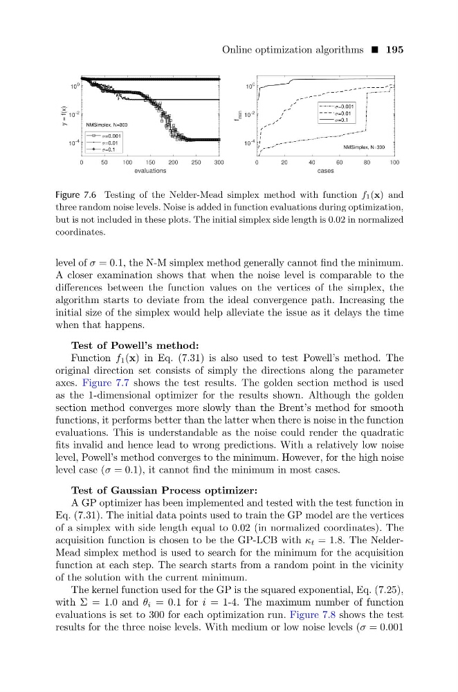
Figure 7.6 Testing of the Nelder-Mead simplex method with function f1(x) and
three random noise levels. Noise is added in function evaluations during optimization,
but is not included in these plots. The initial simplex side length is 0.02 in normalized
coordinates.
level of σ = 0.1, the N-M simplex method generally cannot find the minimum.
A closer examination shows that when the noise level is comparable to the
differences between the function values on the vertices of the simplex, the
algorithm starts to deviate from the ideal convergence path. Increasing the
initial size of the simplex would help alleviate the issue as it delays the time
when that happens.
Test of Powell’s method:
Function f 1 (x) in Eq. (7.31) is also used to test Powell’s method. The
original direction set consists of simply the directions along the parameter
axes. Figure 7.7 shows the test results. The golden section method is used
as the 1-dimensional optimizer for the results shown. Although the golden
section method converges more slowly than the Brent’s method for smooth
functions, it performs better than the latter when there is noise in the function
evaluations. This is understandable as the noise could render the quadratic
fits invalid and hence lead to wrong predictions. With a relatively low noise
level, Powell’s method converges to the minimum. However, for the high noise
level case (σ = 0.1), it cannot find the minimum in most cases.
Test of Gaussian Process optimizer:
A GP optimizer has been implemented and tested with the test function in
Eq. (7.31). The initial data points used to train the GP model are the vertices
of a simplex with side length equal to 0.02 (in normalized coordinates). The
acquisition function is chosen to be the GP-LCB with κ t = 1.8. The NelderMead simplex method is used to search for the minimum for the acquisition
function at each step. The search starts from a random point in the vicinity
of the solution with the current minimum.
The kernel function used for the GP is the squared exponential, Eq. (7.25),
with Σ = 1.0 and θ i = 0.1 for i = 1-4. The maximum number of function
evaluations is set to 300 for each optimization run. Figure 7.8 shows the test
results for the three noise levels. With medium or low noise levels (σ = 0.001
0
50
100
150
200
250
300
evaluations
10
-4
10
-2
10
0
y = f(x)
NMSimplex, N=300
=0.001
=0.01
=0.1
0
20
40
60
80
100
cases
10
-4
10
-2
10
0
f
min
NMSimplex, N=300
=0.001
=0.01
=0.1
Figure 7.6 Testing of the Nelder-Mead simplex method with function f1(x) and
three random noise levels. Noise is added in function evaluations during optimization,
but is not included in these plots. The initial simplex side length is 0.02 in normalized
coordinates.
level of σ = 0.1, the N-M simplex method generally cannot find the minimum.
A closer examination shows that when the noise level is comparable to the
differences between the function values on the vertices of the simplex, the
algorithm starts to deviate from the ideal convergence path. Increasing the
initial size of the simplex would help alleviate the issue as it delays the time
when that happens.
Test of Powell’s method:
Function f 1 (x) in Eq. (7.31) is also used to test Powell’s method. The
original direction set consists of simply the directions along the parameter
axes. Figure 7.7 shows the test results. The golden section method is used
as the 1-dimensional optimizer for the results shown. Although the golden
section method converges more slowly than the Brent’s method for smooth
functions, it performs better than the latter when there is noise in the function
evaluations. This is understandable as the noise could render the quadratic
fits invalid and hence lead to wrong predictions. With a relatively low noise
level, Powell’s method converges to the minimum. However, for the high noise
level case (σ = 0.1), it cannot find the minimum in most cases.
Test of Gaussian Process optimizer:
A GP optimizer has been implemented and tested with the test function in
Eq. (7.31). The initial data points used to train the GP model are the vertices
of a simplex with side length equal to 0.02 (in normalized coordinates). The
acquisition function is chosen to be the GP-LCB with κ t = 1.8. The NelderMead simplex method is used to search for the minimum for the acquisition
function at each step. The search starts from a random point in the vicinity
of the solution with the current minimum.
The kernel function used for the GP is the squared exponential, Eq. (7.25),
with Σ = 1.0 and θ i = 0.1 for i = 1-4. The maximum number of function
evaluations is set to 300 for each optimization run. Figure 7.8 shows the test
results for the three noise levels. With medium or low noise levels (σ = 0.001