Basics of beam dynamics 7
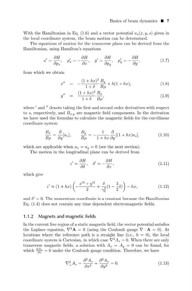
With the Hamiltonian in Eq. (1.6) and a vector potential a s (x, y, s) given in
the local coordinate system, the beam motion can be determined.
The equations of motion for the transverse plane can be derived from the
Hamiltonian, using Hamilton’s equations
x
=
∂H
∂p x
, p
x = −
∂H
∂x
, y
=
∂H
∂p y
, p
y = −
∂H
∂y
,
(1.7)
from which we obtain
x
= −
(1 + hx)
2
1 + δ
B y
Bρ
+ h(1 + hx),
(1.8)
y
=
(1 + hx)
2
1 + δ
B x
Bρ
,
(1.9)
where
and
denote taking the first and second order derivatives with respect
to s, respectively, and B x,y are magnetic field components. In the derivation
we have used the formulas to calculate the magnetic fields for the curvilinear
coordinate system
B x
Bρ
=
∂
∂y
[a s ],
B y
Bρ
= −
1
1 + hx
∂
∂y
[(1 + hx)a s ],
(1.10)
which are applicable when a x = a y = 0 (see the next section).
The motion in the longitudinal plane can be derived from
z
=
∂H
∂δ
, δ
= −
∂H
∂z
,
(1.11)
which give
z
≈ (1 + hx)
−
x
2 + y
2
2
+
δ
γ 2
0
(1 −
3
2
δ)
− hx,
(1.12)
and δ
= 0. The momentum coordinate is a constant because the Hamiltonian
Eq. (1.4) does not contain any time dependent electromagnetic fields.
1.1.2 Magnets and magnetic fields
In the current free region of a static magnetic field, the vector potential satisfies
the Laplace equation, ∇
2 A = 0 (using the Coulomb gauge ∇ · A = 0). At
locations where the reference path is a straight line (i.e., h = 0), the local
coordinate system is Cartesian, in which case ∇
2 A s = 0. When there are only
transverse magnetic fields, a solution with A x = A y = 0 can be found, for
which
∂As
∂s = 0 under the Coulomb gauge condition. Therefore, we have
∇
2
⊥ A s =
∂
2 A s
∂x 2 +
∂
2 A s
∂y 2 = 0.
(1.13)