

6 Beam-based Correction and Optimization for Accelerators
It is customary to change the coordinates from the global system to the
local system through a series of canonical transformations and a change of free
variable from the time t to the path length s. The details of the procedure are
omitted here; interested readers can find the details in Ref. [121]. A reference
particle is assumed to travel on the reference path, with a constant canonical
momentum, P 0 , and its arrival time at location s is t 0 (s). The dynamical
system is measured with canonical coordinates (x, p x , y, p y , ∆z, δ), with the
transverse momentum coordinates normalized by the canonical momentum of
the reference particle
p x =
P x
P 0
≈ x
(1 + δ),
p y =
P y
P 0
≈ y
(1 + δ),
(1.2)
where P x are P y projections of the canonical momentum, P, on the x and y
directions, respectively, x
=
dx
ds , y
=
dy
ds , and the longitudinal coordinates are
∆z = −β 0 c(t − t 0 ),
δ =
P − P 0
P 0
,
(1.3)
where β 0 c is the velocity of the reference particle. Coordinate ∆z is the distance between the particle and the reference particle, with ∆z < 0 indicating
that the particle is behind the reference particle.
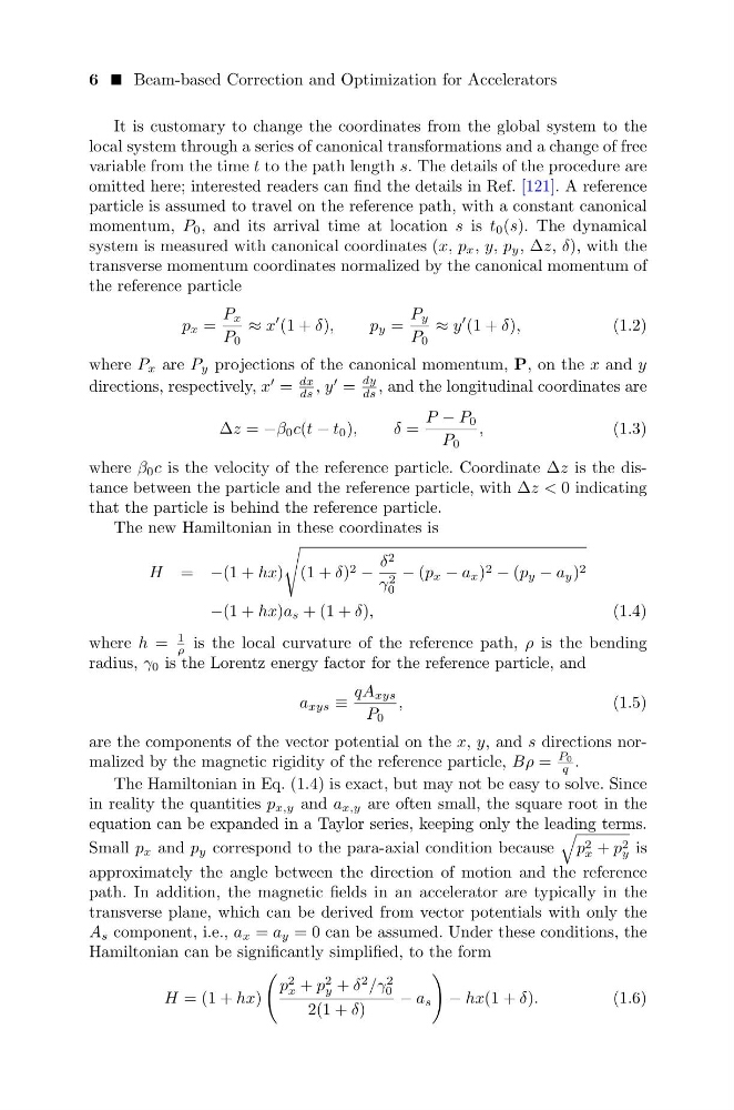
The new Hamiltonian in these coordinates is
H = −(1 + hx)
(1 + δ) 2 −
δ 2
γ 2
0
− (p x − a x ) 2 − (p y − a y ) 2
−(1 + hx)a s + (1 + δ),
(1.4)
where h =
1
ρ is the local curvature of the reference path, ρ is the bending
radius, γ 0 is the Lorentz energy factor for the reference particle, and
a xys ≡
qA xys
P 0
,
(1.5)
are the components of the vector potential on the x, y, and s directions normalized by the magnetic rigidity of the reference particle, Bρ =
P0
q .
The Hamiltonian in Eq. (1.4) is exact, but may not be easy to solve. Since
in reality the quantities p x,y and a x,y are often small, the square root in the
equation can be expanded in a Taylor series, keeping only the leading terms.
Small p x and p y correspond to the para-axial condition because
p 2
x + p 2
y is
approximately the angle between the direction of motion and the reference
path. In addition, the magnetic fields in an accelerator are typically in the
transverse plane, which can be derived from vector potentials with only the
A s component, i.e., a x = a y = 0 can be assumed. Under these conditions, the
Hamiltonian can be significantly simplified, to the form
H = (1 + hx)
p
2
x + p
2
y + δ
2 /γ
2
0
2(1 + δ)
− a s
− hx(1 + δ).
(1.6)
It is customary to change the coordinates from the global system to the
local system through a series of canonical transformations and a change of free
variable from the time t to the path length s. The details of the procedure are
omitted here; interested readers can find the details in Ref. [121]. A reference
particle is assumed to travel on the reference path, with a constant canonical
momentum, P 0 , and its arrival time at location s is t 0 (s). The dynamical
system is measured with canonical coordinates (x, p x , y, p y , ∆z, δ), with the
transverse momentum coordinates normalized by the canonical momentum of
the reference particle
p x =
P x
P 0
≈ x
(1 + δ),
p y =
P y
P 0
≈ y
(1 + δ),
(1.2)
where P x are P y projections of the canonical momentum, P, on the x and y
directions, respectively, x
=
dx
ds , y
=
dy
ds , and the longitudinal coordinates are
∆z = −β 0 c(t − t 0 ),
δ =
P − P 0
P 0
,
(1.3)
where β 0 c is the velocity of the reference particle. Coordinate ∆z is the distance between the particle and the reference particle, with ∆z < 0 indicating
that the particle is behind the reference particle.
The new Hamiltonian in these coordinates is
H = −(1 + hx)
(1 + δ) 2 −
δ 2
γ 2
0
− (p x − a x ) 2 − (p y − a y ) 2
−(1 + hx)a s + (1 + δ),
(1.4)
where h =
1
ρ is the local curvature of the reference path, ρ is the bending
radius, γ 0 is the Lorentz energy factor for the reference particle, and
a xys ≡
qA xys
P 0
,
(1.5)
are the components of the vector potential on the x, y, and s directions normalized by the magnetic rigidity of the reference particle, Bρ =
P0
q .
The Hamiltonian in Eq. (1.4) is exact, but may not be easy to solve. Since
in reality the quantities p x,y and a x,y are often small, the square root in the
equation can be expanded in a Taylor series, keeping only the leading terms.
Small p x and p y correspond to the para-axial condition because
p 2
x + p 2
y is
approximately the angle between the direction of motion and the reference
path. In addition, the magnetic fields in an accelerator are typically in the
transverse plane, which can be derived from vector potentials with only the
A s component, i.e., a x = a y = 0 can be assumed. Under these conditions, the
Hamiltonian can be significantly simplified, to the form
H = (1 + hx)
p
2
x + p
2
y + δ
2 /γ
2
0
2(1 + δ)
− a s
− hx(1 + δ).
(1.6)