

Linear optics measurement and correction - I 101
where g x,y are the horizontal and vertical BPM gains, respectively, φ is the
rotation angle about the s-axis, and C is called the crunch coefficient, which
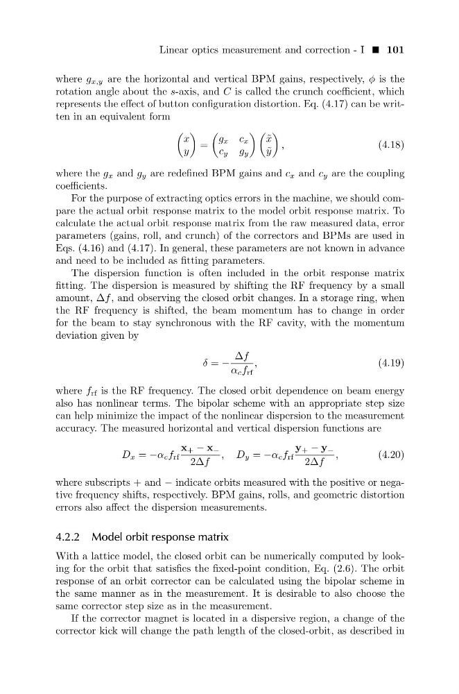
represents the effect of button configuration distortion. Eq. (4.17) can be written in an equivalent form
x
y
=
g x c x
c y g y
˜
x
˜
y
,
(4.18)
where the g x and g y are redefined BPM gains and c x and c y are the coupling
coefficients.
For the purpose of extracting optics errors in the machine, we should compare the actual orbit response matrix to the model orbit response matrix. To
calculate the actual orbit response matrix from the raw measured data, error
parameters (gains, roll, and crunch) of the correctors and BPMs are used in
Eqs. (4.16) and (4.17). In general, these parameters are not known in advance
and need to be included as fitting parameters.
The dispersion function is often included in the orbit response matrix
fitting. The dispersion is measured by shifting the RF frequency by a small
amount, ∆f , and observing the closed orbit changes. In a storage ring, when
the RF frequency is shifted, the beam momentum has to change in order
for the beam to stay synchronous with the RF cavity, with the momentum
deviation given by
δ = −
∆f
α c f rf
,
(4.19)
where f rf is the RF frequency. The closed orbit dependence on beam energy
also has nonlinear terms. The bipolar scheme with an appropriate step size
can help minimize the impact of the nonlinear dispersion to the measurement
accuracy. The measured horizontal and vertical dispersion functions are
D x = −α c f rf
x + − x −
2∆f
, D y = −α c f rf
y + − y −
2∆f
,
(4.20)
where subscripts + and − indicate orbits measured with the positive or negative frequency shifts, respectively. BPM gains, rolls, and geometric distortion
errors also affect the dispersion measurements.
4.2.2 Model orbit response matrix
With a lattice model, the closed orbit can be numerically computed by looking for the orbit that satisfies the fixed-point condition, Eq. (2.6). The orbit
response of an orbit corrector can be calculated using the bipolar scheme in
the same manner as in the measurement. It is desirable to also choose the
same corrector step size as in the measurement.
If the corrector magnet is located in a dispersive region, a change of the
corrector kick will change the path length of the closed-orbit, as described in
where g x,y are the horizontal and vertical BPM gains, respectively, φ is the
rotation angle about the s-axis, and C is called the crunch coefficient, which
represents the effect of button configuration distortion. Eq. (4.17) can be written in an equivalent form
x
y
=
g x c x
c y g y
˜
x
˜
y
,
(4.18)
where the g x and g y are redefined BPM gains and c x and c y are the coupling
coefficients.
For the purpose of extracting optics errors in the machine, we should compare the actual orbit response matrix to the model orbit response matrix. To
calculate the actual orbit response matrix from the raw measured data, error
parameters (gains, roll, and crunch) of the correctors and BPMs are used in
Eqs. (4.16) and (4.17). In general, these parameters are not known in advance
and need to be included as fitting parameters.
The dispersion function is often included in the orbit response matrix
fitting. The dispersion is measured by shifting the RF frequency by a small
amount, ∆f , and observing the closed orbit changes. In a storage ring, when
the RF frequency is shifted, the beam momentum has to change in order
for the beam to stay synchronous with the RF cavity, with the momentum
deviation given by
δ = −
∆f
α c f rf
,
(4.19)
where f rf is the RF frequency. The closed orbit dependence on beam energy
also has nonlinear terms. The bipolar scheme with an appropriate step size
can help minimize the impact of the nonlinear dispersion to the measurement
accuracy. The measured horizontal and vertical dispersion functions are
D x = −α c f rf
x + − x −
2∆f
, D y = −α c f rf
y + − y −
2∆f
,
(4.20)
where subscripts + and − indicate orbits measured with the positive or negative frequency shifts, respectively. BPM gains, rolls, and geometric distortion
errors also affect the dispersion measurements.
4.2.2 Model orbit response matrix
With a lattice model, the closed orbit can be numerically computed by looking for the orbit that satisfies the fixed-point condition, Eq. (2.6). The orbit
response of an orbit corrector can be calculated using the bipolar scheme in
the same manner as in the measurement. It is desirable to also choose the
same corrector step size as in the measurement.
If the corrector magnet is located in a dispersive region, a change of the
corrector kick will change the path length of the closed-orbit, as described in