

Orbit and trajectory correction 87
v
1
-0.5
0
0.5
SVD v-vector
harmonic knob
corrector index
0
10
20
30
40
50
60
v
2
-0.5
0
0.5
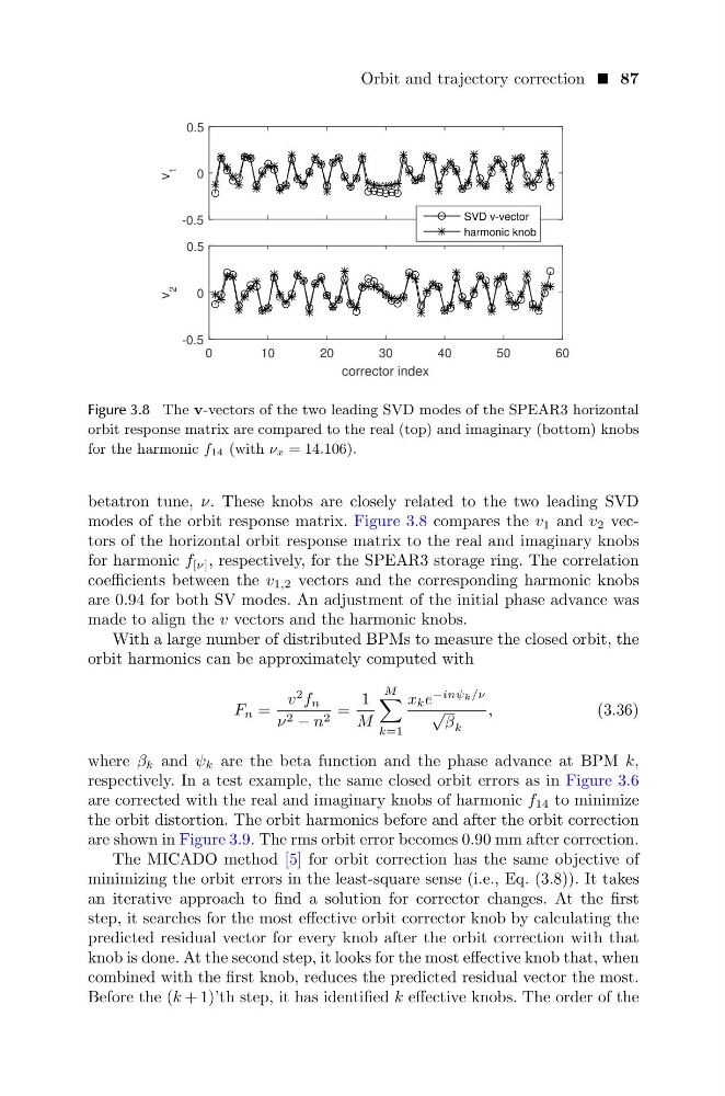
Figure 3.8 The v-vectors of the two leading SVD modes of the SPEAR3 horizontal
orbit response matrix are compared to the real (top) and imaginary (bottom) knobs
for the harmonic f14 (with νx = 14.106).
betatron tune, ν. These knobs are closely related to the two leading SVD
modes of the orbit response matrix. Figure 3.8 compares the v 1 and v 2 vectors of the horizontal orbit response matrix to the real and imaginary knobs
for harmonic f [ν] , respectively, for the SPEAR3 storage ring. The correlation
coefficients between the v 1,2 vectors and the corresponding harmonic knobs
are 0.94 for both SV modes. An adjustment of the initial phase advance was
made to align the v vectors and the harmonic knobs.
With a large number of distributed BPMs to measure the closed orbit, the
orbit harmonics can be approximately computed with
F n =
v
2 f n
ν 2 − n 2 =
1
M
M
k=1
x k e
−inψ k /ν
√
β k
,
(3.36)
where β k and ψ k are the beta function and the phase advance at BPM k,
respectively. In a test example, the same closed orbit errors as in Figure 3.6
are corrected with the real and imaginary knobs of harmonic f 14 to minimize
the orbit distortion. The orbit harmonics before and after the orbit correction
are shown in Figure 3.9. The rms orbit error becomes 0.90 mm after correction.
The MICADO method [5] for orbit correction has the same objective of
minimizing the orbit errors in the least-square sense (i.e., Eq. (3.8)). It takes
an iterative approach to find a solution for corrector changes. At the first
step, it searches for the most effective orbit corrector knob by calculating the
predicted residual vector for every knob after the orbit correction with that
knob is done. At the second step, it looks for the most effective knob that, when
combined with the first knob, reduces the predicted residual vector the most.
Before the (k + 1)’th step, it has identified k effective knobs. The order of the
v
1
-0.5
0
0.5
SVD v-vector
harmonic knob
corrector index
0
10
20
30
40
50
60
v
2
-0.5
0
0.5
Figure 3.8 The v-vectors of the two leading SVD modes of the SPEAR3 horizontal
orbit response matrix are compared to the real (top) and imaginary (bottom) knobs
for the harmonic f14 (with νx = 14.106).
betatron tune, ν. These knobs are closely related to the two leading SVD
modes of the orbit response matrix. Figure 3.8 compares the v 1 and v 2 vectors of the horizontal orbit response matrix to the real and imaginary knobs
for harmonic f [ν] , respectively, for the SPEAR3 storage ring. The correlation
coefficients between the v 1,2 vectors and the corresponding harmonic knobs
are 0.94 for both SV modes. An adjustment of the initial phase advance was
made to align the v vectors and the harmonic knobs.
With a large number of distributed BPMs to measure the closed orbit, the
orbit harmonics can be approximately computed with
F n =
v
2 f n
ν 2 − n 2 =
1
M
M
k=1
x k e
−inψ k /ν
√
β k
,
(3.36)
where β k and ψ k are the beta function and the phase advance at BPM k,
respectively. In a test example, the same closed orbit errors as in Figure 3.6
are corrected with the real and imaginary knobs of harmonic f 14 to minimize
the orbit distortion. The orbit harmonics before and after the orbit correction
are shown in Figure 3.9. The rms orbit error becomes 0.90 mm after correction.
The MICADO method [5] for orbit correction has the same objective of
minimizing the orbit errors in the least-square sense (i.e., Eq. (3.8)). It takes
an iterative approach to find a solution for corrector changes. At the first
step, it searches for the most effective orbit corrector knob by calculating the
predicted residual vector for every knob after the orbit correction with that
knob is done. At the second step, it looks for the most effective knob that, when
combined with the first knob, reduces the predicted residual vector the most.
Before the (k + 1)’th step, it has identified k effective knobs. The order of the