

1 3
Top Curr Chem (Z) (2018) 376:24
the calculations, as undesired effects due to the temporal overlap of the pulses do not
need to be considered. Furthermore, the obscuring of any coherent dynamics, which
occurs on the same timescale as the duration of the pulses, is avoided, and the highest possible temporal resolution is achieved. The impulsive limit has been adopted
throughout this review.
Simulation protocols for nonlinear optical spectroscopy deal with solving Eq. (7)
or, more generally, Eq. 8 when working with realistic pulse shapes. This requires
computing the interactions of the system with three time-dependent electric fields
as well as its field-free evolution between them. In principle, Eq. 7 could be solved
without any approximation, given knowledge of the multidimensional potentials
associated with each electronic state involved in the evolution of the density matrix,
enabling propagation of populations and coherences. In this case, non-adiabatic
couplings and transition dipole moments along the potential energy surfaces (PES)
would be required to allow population transfer and interaction with the field, respectively. It would then be possible to treat electronic and nuclear degrees of freedom fully quantum-mechanically by quantum dynamics, thereby resolving coherent oscillatory dynamics, line broadening (due to finite excited-state lifetimes) and
vibrational progressions due to wave packet decoherence and recoherence. Furthermore, arbitrary pulses could be straightforwardly incorporated into the simulations,
providing an opportunity to study the effects of the pulse’s central frequency, bandwidth and polarization [36, 37].
The drawback to quantum dynamics simulations is the high cost of pre-computing the PES, a task that quickly becomes infeasible with an increasing number of
degrees of freedom. As a workaround, simulations are often run on parameterized
two- or three-dimensional potentials that approximate the exact PES through analytical expressions, with parameters chosen to fit the energetics of a few representative points along the PES. This approach was recently applied to simulate 2DES in
Rhodopsin [38]. Methods such as multi-configuration time-dependent Hartree have
facilitated simulations on multidimensional surfaces [39].
Another approach for solving Eqs. (7) and (8) involves the stochastic modeling
of bath fluctuations in a semi-classical fashion (stochastic Liouville equations, SLE)
[40, 41]. At the heart of SLE is the explicit inclusion of collective bath modes in the
system’s Hamiltonian. The Hamiltonian is formally time-independent, but depends
on some classical time-dependent stochastic variables σ(t), which represent the bath.
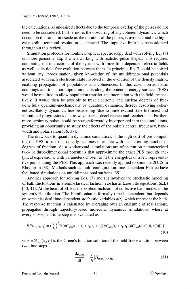
The response function is calculated by averaging over an ensemble of realizations,
propagated through trajectory-based molecular dynamics simulations, where at
every subsequent time-step it is evaluated as
where G (t) ( i , j ) is the Green’s function solution of the field-free evolution between
two time steps
(10)
R
(3) (t 1 , t 2 , t 3 ) =
i
�
3
Tr[ ̂
í µí¼G í µí¼(t) (t 3 + t 2 + t 1 , t 2 + t 1 )[ ̂
í µí¼G í µí¼(t) (t 2 + t 1 , t 1 )[ ̂
í µí¼G í µí¼(t) (t 1 , 0)[ ̂
í µí¼, í µí¼(0)]]]]
(11)
d ̂
í µí¼ í µí¼(t)
dt
=
i
�
̂
H 0;í µí¼(t) , í µí¼ í µí¼(t)
71
Reprinted from the journal
Top Curr Chem (Z) (2018) 376:24
the calculations, as undesired effects due to the temporal overlap of the pulses do not
need to be considered. Furthermore, the obscuring of any coherent dynamics, which
occurs on the same timescale as the duration of the pulses, is avoided, and the highest possible temporal resolution is achieved. The impulsive limit has been adopted
throughout this review.
Simulation protocols for nonlinear optical spectroscopy deal with solving Eq. (7)
or, more generally, Eq. 8 when working with realistic pulse shapes. This requires
computing the interactions of the system with three time-dependent electric fields
as well as its field-free evolution between them. In principle, Eq. 7 could be solved
without any approximation, given knowledge of the multidimensional potentials
associated with each electronic state involved in the evolution of the density matrix,
enabling propagation of populations and coherences. In this case, non-adiabatic
couplings and transition dipole moments along the potential energy surfaces (PES)
would be required to allow population transfer and interaction with the field, respectively. It would then be possible to treat electronic and nuclear degrees of freedom fully quantum-mechanically by quantum dynamics, thereby resolving coherent oscillatory dynamics, line broadening (due to finite excited-state lifetimes) and
vibrational progressions due to wave packet decoherence and recoherence. Furthermore, arbitrary pulses could be straightforwardly incorporated into the simulations,
providing an opportunity to study the effects of the pulse’s central frequency, bandwidth and polarization [36, 37].
The drawback to quantum dynamics simulations is the high cost of pre-computing the PES, a task that quickly becomes infeasible with an increasing number of
degrees of freedom. As a workaround, simulations are often run on parameterized
two- or three-dimensional potentials that approximate the exact PES through analytical expressions, with parameters chosen to fit the energetics of a few representative points along the PES. This approach was recently applied to simulate 2DES in
Rhodopsin [38]. Methods such as multi-configuration time-dependent Hartree have
facilitated simulations on multidimensional surfaces [39].
Another approach for solving Eqs. (7) and (8) involves the stochastic modeling
of bath fluctuations in a semi-classical fashion (stochastic Liouville equations, SLE)
[40, 41]. At the heart of SLE is the explicit inclusion of collective bath modes in the
system’s Hamiltonian. The Hamiltonian is formally time-independent, but depends
on some classical time-dependent stochastic variables σ(t), which represent the bath.
The response function is calculated by averaging over an ensemble of realizations,
propagated through trajectory-based molecular dynamics simulations, where at
every subsequent time-step it is evaluated as
where G (t) ( i , j ) is the Green’s function solution of the field-free evolution between
two time steps
(10)
R
(3) (t 1 , t 2 , t 3 ) =
i
�
3
Tr[ ̂
í µí¼G í µí¼(t) (t 3 + t 2 + t 1 , t 2 + t 1 )[ ̂
í µí¼G í µí¼(t) (t 2 + t 1 , t 1 )[ ̂
í µí¼G í µí¼(t) (t 1 , 0)[ ̂
í µí¼, í µí¼(0)]]]]
(11)
d ̂
í µí¼ í µí¼(t)
dt
=
i
�
̂
H 0;í µí¼(t) , í µí¼ í µí¼(t)
71
Reprinted from the journal