

Top Curr Chem (Z) (2018) 376:24
1 3
Since bath dynamics is non-Markovian, solving Eq. 10 requires knowledge of
the past evolution of the system. Bulk-induced dephasing effects are automatically
included via ensemble averaging. Trajectory-based approaches face the challenge of
the computational cost associated with the propagation of a swarm of trajectories
(particularly those in the excited state) and the absence of a well-defined density
matrix responsible for the quantum feedback on the classical bath during a coherence state evolution. Various trajectory-based implementations that address these
issues have been documented in recent years [42–45].
For systems with a classical bath following Gaussian statistics and linear system–bath coupling, Eqs. (8) can be solved using the second-order cumulant expansion, i.e. the cumulant expansion of Gaussian fluctuations (CGF) [46]. This method
makes it possible to calculate the shapes of electronic transition bands coupled to a
bath (for fluctuations with arbitrary timescales) using the formalism of line shape
functions, g ij (t); see Appendix for details. Within the CGF framework, the population transfer can be accounted for phenomenologically according to the Lindblad
equation (see Appendix), with secular approximation to the Green’s function enabling partitioning of the nonlinear response (Eqs. 9, 10) into population and coherence contributions. For instance, considering the manifold of ground (g) and excited
(e, f) states, and just the ESAs detected in the rephasing phase-matching direction
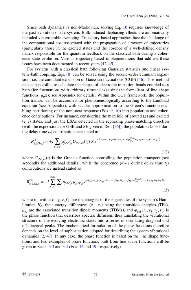
(with the expressions for GSB and SE given in Ref. [36]), the population (e’ = e during delay time t 2 ) contributions are stated as
where G e � e � ,ee (t) is the Green’s function controlling the population transport (see
Appendix for additional details), while the coherence (e′≠ e during delay time t 2 )
contributions are instead stated as
where ε a , with a ∈ {g, e, f } , are the energies of the eigenstates of the system’s Hamiltonian H 0 , their energy differences (ε a − ε b ) being the transition energies (TEs),
μ ab are the associated transition dipole moments (TDMs), and e � fe ( 4 , 3 , 2 , 1 ) is
the phase function that describes spectral diffusion, thus translating the vibrational
structure of the evolving electronic states into a series of oscillating diagonal and
off-diagonal peaks. The mathematical formulation of the phase functions therefore
depends on the level of sophistication adopted for describing the system vibrational
dynamics [2, 47]. In any case, the phase function is based on the line shape functions, and two examples of phase functions built from line shape functions will be
given in Sects. 3.3 and 3.4 (Eqs. 16 and 19, respectively).
(12)
R
(3)
k 1 ESA,i
= +i
∑
e � ,e,f
2
fe �
2
ge
G e � e � ,ee (t 2 ) × e
−i( f − e � )t 3 +( e − g )t 1 +
ESA,i
fe � e
(t 1 ,t 1 +t 2 ,t 1 +t 2 +t 3 ,0)
(13)
R
(3)
k 1 ESA,ii
= +i
e�≠e
∑
e � ,e f
∑
f
fe� fe ge� ge e
−i( f − e )t 3 × e
−i( e� − e )t 2 +( e − g )t 1 +
ESA,ii
fe�e
(t 1 ,t 1 +t 2 ,t 1 +t 2 +t 3 ,0)
72
Reprinted from the journal
1 3
Since bath dynamics is non-Markovian, solving Eq. 10 requires knowledge of
the past evolution of the system. Bulk-induced dephasing effects are automatically
included via ensemble averaging. Trajectory-based approaches face the challenge of
the computational cost associated with the propagation of a swarm of trajectories
(particularly those in the excited state) and the absence of a well-defined density
matrix responsible for the quantum feedback on the classical bath during a coherence state evolution. Various trajectory-based implementations that address these
issues have been documented in recent years [42–45].
For systems with a classical bath following Gaussian statistics and linear system–bath coupling, Eqs. (8) can be solved using the second-order cumulant expansion, i.e. the cumulant expansion of Gaussian fluctuations (CGF) [46]. This method
makes it possible to calculate the shapes of electronic transition bands coupled to a
bath (for fluctuations with arbitrary timescales) using the formalism of line shape
functions, g ij (t); see Appendix for details. Within the CGF framework, the population transfer can be accounted for phenomenologically according to the Lindblad
equation (see Appendix), with secular approximation to the Green’s function enabling partitioning of the nonlinear response (Eqs. 9, 10) into population and coherence contributions. For instance, considering the manifold of ground (g) and excited
(e, f) states, and just the ESAs detected in the rephasing phase-matching direction
(with the expressions for GSB and SE given in Ref. [36]), the population (e’ = e during delay time t 2 ) contributions are stated as
where G e � e � ,ee (t) is the Green’s function controlling the population transport (see
Appendix for additional details), while the coherence (e′≠ e during delay time t 2 )
contributions are instead stated as
where ε a , with a ∈ {g, e, f } , are the energies of the eigenstates of the system’s Hamiltonian H 0 , their energy differences (ε a − ε b ) being the transition energies (TEs),
μ ab are the associated transition dipole moments (TDMs), and e � fe ( 4 , 3 , 2 , 1 ) is
the phase function that describes spectral diffusion, thus translating the vibrational
structure of the evolving electronic states into a series of oscillating diagonal and
off-diagonal peaks. The mathematical formulation of the phase functions therefore
depends on the level of sophistication adopted for describing the system vibrational
dynamics [2, 47]. In any case, the phase function is based on the line shape functions, and two examples of phase functions built from line shape functions will be
given in Sects. 3.3 and 3.4 (Eqs. 16 and 19, respectively).
(12)
R
(3)
k 1 ESA,i
= +i
∑
e � ,e,f
2
fe �
2
ge
G e � e � ,ee (t 2 ) × e
−i( f − e � )t 3 +( e − g )t 1 +
ESA,i
fe � e
(t 1 ,t 1 +t 2 ,t 1 +t 2 +t 3 ,0)
(13)
R
(3)
k 1 ESA,ii
= +i
e�≠e
∑
e � ,e f
∑
f
fe� fe ge� ge e
−i( f − e )t 3 × e
−i( e� − e )t 2 +( e − g )t 1 +
ESA,ii
fe�e
(t 1 ,t 1 +t 2 ,t 1 +t 2 +t 3 ,0)
72
Reprinted from the journal