

Top Curr Chem (Z) (2018) 376:24
1 3
, is included in the system Hamiltonian, i.e. ̂
H = ̂
H 0 + ̂
H
� (t) . The density matrix is
expanded as
where the superscript denotes the nth-order expansion. In this perturbative scheme,
the Liouville-von Neumann equation can be solved by sorting in powers of ̂
í µí¼ , followed by an iterative integration of the resulting equations (see Appendix for the
explicit form of the third-order density matrix).
Writing out the perturbation (Eq. 5) and reformulating the density matrix as a function of the time intervals t i between the pulses
(with
t 1 = 2 − 1 , t 2 = 3 − 2 , t 3 = t − 3 ),
the
nth-order
polarization
P
(n) (t) =
⟨
̂
í µí¼ ̂
í µí¼
(n) (t)
⟩
= Tr
⌊
̂
í µí¼ ̂
í µí¼
(n) (t)
⌋ becomes third-order,
where the system-specific (third-order) response R
(3)
(t 1 ,t 2 ,t 3 )
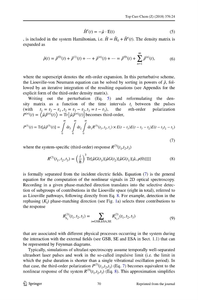
is formally separated from the incident electric fields. Equation (7) is the general
equation for the computation of the nonlinear signals in 2D optical spectroscopy.
Recording in a given phase-matched direction translates into the selective detection of subgroups of contributions in the Liouville space (eight in total), referred to
as Liouville pathways, following directly from Eq. 8. For example, detection in the
rephasing (K I ) phase-matching direction (see Fig. 1a) selects three contributions to
the response
that are associated with different physical processes occurring in the system during
the interaction with the external fields (see GSB, SE and ESA in Sect. 1.1) that can
be represented by Feynman diagrams.
Typically, simulations of ultrafast spectroscopy assume temporally well-separated
ultrashort laser pulses and work in the so-called impulsive limit (i.e. the limit in
which the pulse duration is shorter than a single vibrational oscillation period). In
that case, the third-order polarization P
(3)
(t 1 ,t 2 ,t 3 ) (Eq. 7) becomes equivalent to the
nonlinear response of the system R
(3)
(t 1 ,t 2 ,t 3 ) (Eq. 8). This approximation simplifies
(5)
̂
H
� (t) = − ̂
í µí¼ ⋅ E(t)
(6)
̂
í µí¼(t) = ̂
í µí¼
(0) (t) + ̂
í µí¼
(1) (t) + ⋯ + ̂
í µí¼
(n) (t) + ⋯ = ̂
í µí¼
(0) (t) +
∞
∑
n=1
̂
í µí¼
(n) (t),
(7)
P
(3) (t) = Tr[ ̂
í µí¼ ̂
í µí¼
(3) (t)] =
∞
∫
0
dt 3
∞
∫
0
dt 2
∞
∫
0
dt 1 R
(3) (t 3 , t 2 , t 1 ) × E(t − t 3 )E(t − t 3 − t 2 )E(t − t 3 t 2 − t 1 )
(8)
R
(3) (t 1 , t 2 , t 3 ) =
i
�
3
Tr[ ̂
í µí¼G(t 3 )[ ̂
í µí¼G(t 2 )[ ̂
í µí¼G(t 1 )[ ̂
í µí¼, í µí¼(0)]]]]
(9)
R
(3)
k 1
(t 1 , t 2 , t 3 ) =
∑
i=GSB,ESA,SE
R
(3)
k 1 ,i
(t 1 , t 2 , t 3 )
70
Reprinted from the journal
1 3
, is included in the system Hamiltonian, i.e. ̂
H = ̂
H 0 + ̂
H
� (t) . The density matrix is
expanded as
where the superscript denotes the nth-order expansion. In this perturbative scheme,
the Liouville-von Neumann equation can be solved by sorting in powers of ̂
í µí¼ , followed by an iterative integration of the resulting equations (see Appendix for the
explicit form of the third-order density matrix).
Writing out the perturbation (Eq. 5) and reformulating the density matrix as a function of the time intervals t i between the pulses
(with
t 1 = 2 − 1 , t 2 = 3 − 2 , t 3 = t − 3 ),
the
nth-order
polarization
P
(n) (t) =
⟨
̂
í µí¼ ̂
í µí¼
(n) (t)
⟩
= Tr
⌊
̂
í µí¼ ̂
í µí¼
(n) (t)
⌋ becomes third-order,
where the system-specific (third-order) response R
(3)
(t 1 ,t 2 ,t 3 )
is formally separated from the incident electric fields. Equation (7) is the general
equation for the computation of the nonlinear signals in 2D optical spectroscopy.
Recording in a given phase-matched direction translates into the selective detection of subgroups of contributions in the Liouville space (eight in total), referred to
as Liouville pathways, following directly from Eq. 8. For example, detection in the
rephasing (K I ) phase-matching direction (see Fig. 1a) selects three contributions to
the response
that are associated with different physical processes occurring in the system during
the interaction with the external fields (see GSB, SE and ESA in Sect. 1.1) that can
be represented by Feynman diagrams.
Typically, simulations of ultrafast spectroscopy assume temporally well-separated
ultrashort laser pulses and work in the so-called impulsive limit (i.e. the limit in
which the pulse duration is shorter than a single vibrational oscillation period). In
that case, the third-order polarization P
(3)
(t 1 ,t 2 ,t 3 ) (Eq. 7) becomes equivalent to the
nonlinear response of the system R
(3)
(t 1 ,t 2 ,t 3 ) (Eq. 8). This approximation simplifies
(5)
̂
H
� (t) = − ̂
í µí¼ ⋅ E(t)
(6)
̂
í µí¼(t) = ̂
í µí¼
(0) (t) + ̂
í µí¼
(1) (t) + ⋯ + ̂
í µí¼
(n) (t) + ⋯ = ̂
í µí¼
(0) (t) +
∞
∑
n=1
̂
í µí¼
(n) (t),
(7)
P
(3) (t) = Tr[ ̂
í µí¼ ̂
í µí¼
(3) (t)] =
∞
∫
0
dt 3
∞
∫
0
dt 2
∞
∫
0
dt 1 R
(3) (t 3 , t 2 , t 1 ) × E(t − t 3 )E(t − t 3 − t 2 )E(t − t 3 t 2 − t 1 )
(8)
R
(3) (t 1 , t 2 , t 3 ) =
i
�
3
Tr[ ̂
í µí¼G(t 3 )[ ̂
í µí¼G(t 2 )[ ̂
í µí¼G(t 1 )[ ̂
í µí¼, í µí¼(0)]]]]
(9)
R
(3)
k 1
(t 1 , t 2 , t 3 ) =
∑
i=GSB,ESA,SE
R
(3)
k 1 ,i
(t 1 , t 2 , t 3 )
70
Reprinted from the journal