

1 3
Top Curr Chem (Z) (2018) 376:24
In the following sections, after presenting the basic theoretical background for
2DES and the approximation frameworks adopted in our studies, we review our
recent efforts in developing computational tools for simulating 2DUV spectra of
two major biological macromolecules, proteins and nucleic acids, focusing on the
chromophoric units that provide absorption distinct from their backbones.
3 Theoretical Background
3.1 Density Matrix Formalism and 2DES Response Functions
A unified theory for nonlinear optical spectroscopy [2] has been developed using
density matrix formalism to represent the state of matter and its evolution in the
Liouville space in order to determine the nonlinear response generated by the
light–matter interactions. As mentioned above, the source of the signal field recorded
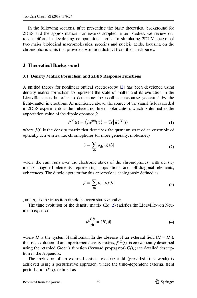
in 2DES experiments is the induced nonlinear polarization, which is defined as the
expectation value of the dipole operator ̂
í µí¼
where ̂
í µí¼(t) is the density matrix that describes the quantum state of an ensemble of
optically active sites, i.e. chromophores (or more generally, molecules)
where the sum runs over the electronic states of the chromophores, with density
matrix diagonal elements representing populations and off-diagonal elements,
coherences. The dipole operator for this ensemble is analogously defined as
, and μ ab is the transition dipole between states a and b.
The time evolution of the density matrix (Eq. 2) satisfies the Liouville-von Neumann equation,
where ̂
H is the system Hamiltonian. In the absence of an external field ( ̂
H = ̂
H 0 ) ,
the free evolution of an unperturbed density matrix, ̂
í µí¼
(0) (t) , is conveniently described
using the retarded Green’s function (forward propagator) G(t); see detailed description in the Appendix.
The inclusion of an external optical electric field (provided it is weak) is
achieved using a perturbative approach, where the time-dependent external field
perturbation ̂
H � (t) , defined as
(1)
P
(n) (t) =
⟨
̂
í µí¼ ̂
í µí¼
(n) (t)
⟩
= Tr
⌊
̂
í µí¼ ̂
í µí¼
(n) (t)
⌋
(2)
̂
í µí¼ =
�
ab
í µí¼ ab �a⟩⟨b�
(3)
̂
í µí¼ =
�
ab
í µí¼ ab �a⟩⟨b�
(4)
i�
d ̂
í µí¼
dt
= [ ̂
H, ̂
í µí¼]
69
Reprinted from the journal
Top Curr Chem (Z) (2018) 376:24
In the following sections, after presenting the basic theoretical background for
2DES and the approximation frameworks adopted in our studies, we review our
recent efforts in developing computational tools for simulating 2DUV spectra of
two major biological macromolecules, proteins and nucleic acids, focusing on the
chromophoric units that provide absorption distinct from their backbones.
3 Theoretical Background
3.1 Density Matrix Formalism and 2DES Response Functions
A unified theory for nonlinear optical spectroscopy [2] has been developed using
density matrix formalism to represent the state of matter and its evolution in the
Liouville space in order to determine the nonlinear response generated by the
light–matter interactions. As mentioned above, the source of the signal field recorded
in 2DES experiments is the induced nonlinear polarization, which is defined as the
expectation value of the dipole operator ̂
í µí¼
where ̂
í µí¼(t) is the density matrix that describes the quantum state of an ensemble of
optically active sites, i.e. chromophores (or more generally, molecules)
where the sum runs over the electronic states of the chromophores, with density
matrix diagonal elements representing populations and off-diagonal elements,
coherences. The dipole operator for this ensemble is analogously defined as
, and μ ab is the transition dipole between states a and b.
The time evolution of the density matrix (Eq. 2) satisfies the Liouville-von Neumann equation,
where ̂
H is the system Hamiltonian. In the absence of an external field ( ̂
H = ̂
H 0 ) ,
the free evolution of an unperturbed density matrix, ̂
í µí¼
(0) (t) , is conveniently described
using the retarded Green’s function (forward propagator) G(t); see detailed description in the Appendix.
The inclusion of an external optical electric field (provided it is weak) is
achieved using a perturbative approach, where the time-dependent external field
perturbation ̂
H � (t) , defined as
(1)
P
(n) (t) =
⟨
̂
í µí¼ ̂
í µí¼
(n) (t)
⟩
= Tr
⌊
̂
í µí¼ ̂
í µí¼
(n) (t)
⌋
(2)
̂
í µí¼ =
�
ab
í µí¼ ab �a⟩⟨b�
(3)
̂
í µí¼ =
�
ab
í µí¼ ab �a⟩⟨b�
(4)
i�
d ̂
í µí¼
dt
= [ ̂
H, ̂
í µí¼]
69
Reprinted from the journal