

73
The bash script is called LVA_(metal)_2018.sh, and it runs four programs in succession:
1. rotcoord – rotates X and Y coordinates in data file 38 degrees to align the data with the
north-south estimation grid required by the LVA programs.
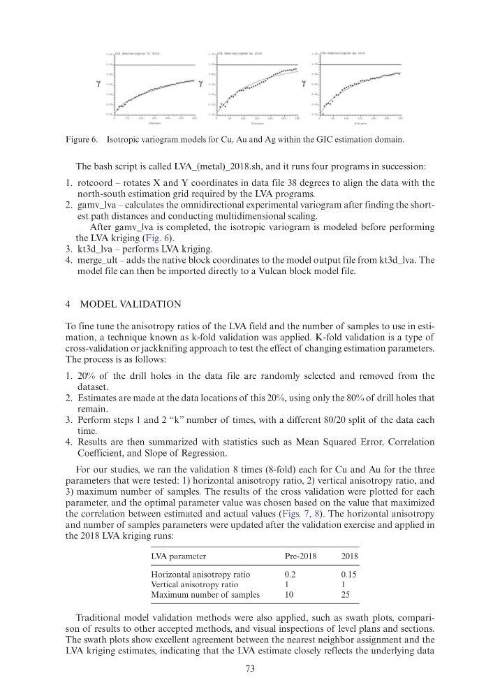
2. gamv_lva – calculates the omnidirectional experimental variogram after finding the shortest path distances and conducting multidimensional scaling.
After gamv_lva is completed, the isotropic variogram is modeled before performing
the LVA kriging (Fig. 6).
3. kt3d_lva – performs LVA kriging.
4. merge_ult – adds the native block coordinates to the model output file from kt3d_lva. The
model file can then be imported directly to a Vulcan block model file.
4 MODEL VALIDATION
To fine tune the anisotropy ratios of the LVA field and the number of samples to use in estimation, a technique known as k-fold validation was applied. K-fold validation is a type of
cross-validation or jackknifing approach to test the effect of changing estimation parameters.
The process is as follows:
1. 20% of the drill holes in the data file are randomly selected and removed from the
dataset.
2. Estimates are made at the data locations of this 20%, using only the 80% of drill holes that
remain.
3. Perform steps 1 and 2 “k” number of times, with a different 80/20 split of the data each
time.
4. Results are then summarized with statistics such as Mean Squared Error, Correlation
Coefficient, and Slope of Regression.
For our studies, we ran the validation 8 times (8-fold) each for Cu and Au for the three
parameters that were tested: 1) horizontal anisotropy ratio, 2) vertical anisotropy ratio, and
3) maximum number of samples. The results of the cross validation were plotted for each
parameter, and the optimal parameter value was chosen based on the value that maximized
the correlation between estimated and actual values (Figs. 7, 8). The horizontal anisotropy
and number of samples parameters were updated after the validation exercise and applied in
the 2018 LVA kriging runs:
LVA parameter
Pre-2018
2018
Horizontal anisotropy ratio
0.2
0.15
Vertical anisotropy ratio
1
1
Maximum number of samples
10
25
Traditional model validation methods were also applied, such as swath plots, comparison of results to other accepted methods, and visual inspections of level plans and sections.
The swath plots show excellent agreement between the nearest neighbor assignment and the
LVA kriging estimates, indicating that the LVA estimate closely reflects the underlying data
Figure 6. Isotropic variogram models for Cu, Au and Ag within the GIC estimation domain.
y
The bash script is called LVA_(metal)_2018.sh, and it runs four programs in succession:
1. rotcoord – rotates X and Y coordinates in data file 38 degrees to align the data with the
north-south estimation grid required by the LVA programs.
2. gamv_lva – calculates the omnidirectional experimental variogram after finding the shortest path distances and conducting multidimensional scaling.
After gamv_lva is completed, the isotropic variogram is modeled before performing
the LVA kriging (Fig. 6).
3. kt3d_lva – performs LVA kriging.
4. merge_ult – adds the native block coordinates to the model output file from kt3d_lva. The
model file can then be imported directly to a Vulcan block model file.
4 MODEL VALIDATION
To fine tune the anisotropy ratios of the LVA field and the number of samples to use in estimation, a technique known as k-fold validation was applied. K-fold validation is a type of
cross-validation or jackknifing approach to test the effect of changing estimation parameters.
The process is as follows:
1. 20% of the drill holes in the data file are randomly selected and removed from the
dataset.
2. Estimates are made at the data locations of this 20%, using only the 80% of drill holes that
remain.
3. Perform steps 1 and 2 “k” number of times, with a different 80/20 split of the data each
time.
4. Results are then summarized with statistics such as Mean Squared Error, Correlation
Coefficient, and Slope of Regression.
For our studies, we ran the validation 8 times (8-fold) each for Cu and Au for the three
parameters that were tested: 1) horizontal anisotropy ratio, 2) vertical anisotropy ratio, and
3) maximum number of samples. The results of the cross validation were plotted for each
parameter, and the optimal parameter value was chosen based on the value that maximized
the correlation between estimated and actual values (Figs. 7, 8). The horizontal anisotropy
and number of samples parameters were updated after the validation exercise and applied in
the 2018 LVA kriging runs:
LVA parameter
Pre-2018
2018
Horizontal anisotropy ratio
0.2
0.15
Vertical anisotropy ratio
1
1
Maximum number of samples
10
25
Traditional model validation methods were also applied, such as swath plots, comparison of results to other accepted methods, and visual inspections of level plans and sections.
The swath plots show excellent agreement between the nearest neighbor assignment and the
LVA kriging estimates, indicating that the LVA estimate closely reflects the underlying data
Figure 6. Isotropic variogram models for Cu, Au and Ag within the GIC estimation domain.
y