

72
The results of this work showed much better replication of the local spatial distribution
of grades due to the improved LVA field. The LVA estimate was validated using standard
approaches and for the first time, the model was used for mine design and reporting of
reserves and resources in December 2014.
3.4.3 2018
In order to more accurately reflect the differences between spatial distributions of Cu and Au,
the LVA field generation method was revisited in early 2018. Dr. Boisvert was again engaged
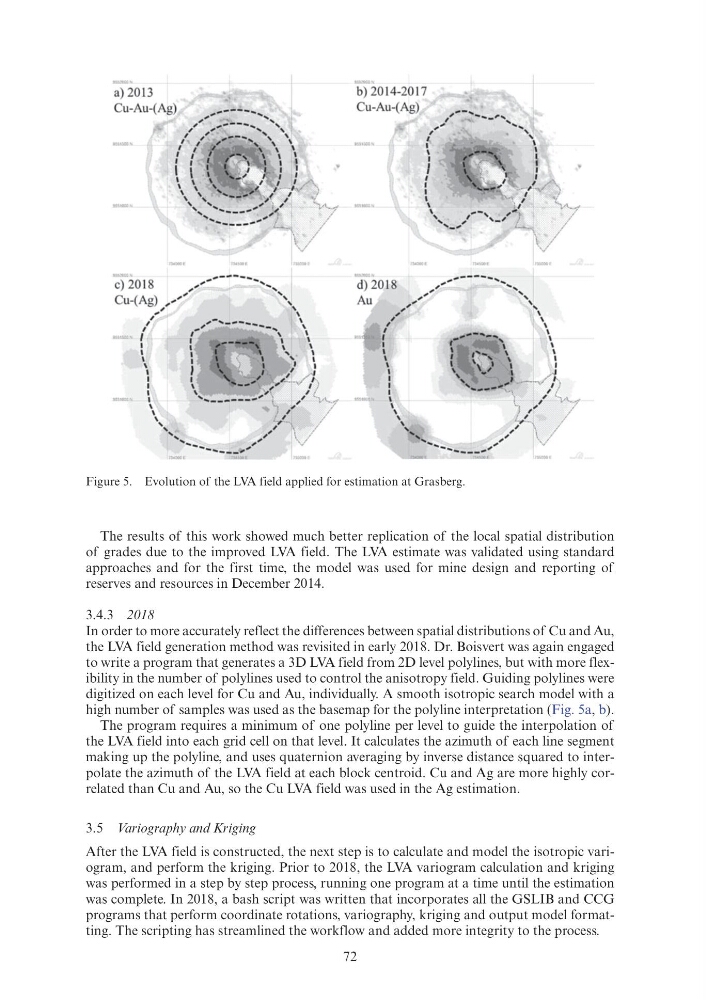
to write a program that generates a 3D LVA field from 2D level polylines, but with more flexibility in the number of polylines used to control the anisotropy field. Guiding polylines were
digitized on each level for Cu and Au, individually. A smooth isotropic search model with a
high number of samples was used as the basemap for the polyline interpretation (Fig. 5a, b).
The program requires a minimum of one polyline per level to guide the interpolation of
the LVA field into each grid cell on that level. It calculates the azimuth of each line segment
making up the polyline, and uses quaternion averaging by inverse distance squared to interpolate the azimuth of the LVA field at each block centroid. Cu and Ag are more highly correlated than Cu and Au, so the Cu LVA field was used in the Ag estimation.
3.5 Variography and Kriging
After the LVA field is constructed, the next step is to calculate and model the isotropic variogram, and perform the kriging. Prior to 2018, the LVA variogram calculation and kriging
was performed in a step by step process, running one program at a time until the estimation
was complete. In 2018, a bash script was written that incorporates all the GSLIB and CCG
programs that perform coordinate rotations, variography, kriging and output model formatting. The scripting has streamlined the workflow and added more integrity to the process.
Figure 5. Evolution of the LVA field applied for estimation at Grasberg.
a) 2013
Cu-Au-(Ag)
'"'''"
•
b) 2014-2017
Cu-Au-(Ag)
d) 2018
Au
The results of this work showed much better replication of the local spatial distribution
of grades due to the improved LVA field. The LVA estimate was validated using standard
approaches and for the first time, the model was used for mine design and reporting of
reserves and resources in December 2014.
3.4.3 2018
In order to more accurately reflect the differences between spatial distributions of Cu and Au,
the LVA field generation method was revisited in early 2018. Dr. Boisvert was again engaged
to write a program that generates a 3D LVA field from 2D level polylines, but with more flexibility in the number of polylines used to control the anisotropy field. Guiding polylines were
digitized on each level for Cu and Au, individually. A smooth isotropic search model with a
high number of samples was used as the basemap for the polyline interpretation (Fig. 5a, b).
The program requires a minimum of one polyline per level to guide the interpolation of
the LVA field into each grid cell on that level. It calculates the azimuth of each line segment
making up the polyline, and uses quaternion averaging by inverse distance squared to interpolate the azimuth of the LVA field at each block centroid. Cu and Ag are more highly correlated than Cu and Au, so the Cu LVA field was used in the Ag estimation.
3.5 Variography and Kriging
After the LVA field is constructed, the next step is to calculate and model the isotropic variogram, and perform the kriging. Prior to 2018, the LVA variogram calculation and kriging
was performed in a step by step process, running one program at a time until the estimation
was complete. In 2018, a bash script was written that incorporates all the GSLIB and CCG
programs that perform coordinate rotations, variography, kriging and output model formatting. The scripting has streamlined the workflow and added more integrity to the process.
Figure 5. Evolution of the LVA field applied for estimation at Grasberg.
a) 2013
Cu-Au-(Ag)
'"'''"
•
b) 2014-2017
Cu-Au-(Ag)
d) 2018
Au