

42
further analysis we calculate the selected measures of dependence for logarithmic returns
of the selected risk factors. In Fig. 3 we highlighted those factors for which the relationship
seems to be the strongest by visual inspection. Based on Fig. 3 we have selected four market risk factors: Cu, Ag, Au and USDPLN. They are presented in Fig. 1. They seem to be
related however the dependence have different character. For some time periods we observe
the positive relationship between the selected factors while for some cases—negative. In the
further analysis we quantify the dependence and prove our assumption by using the appropriate correlation coefficients.
After visual inspection, we propose to quantify the relationship between the selected market risk factors. We propose to take under consideration three different measures of dependence. The first one is the classical Pearson correlation coefficient [1]. In statistics, the Pearson
correlation coefficient is a measure of the linear relation between two variables X and Y.
According to the Cauchy–Schwarz inequality it has a value between +1 and −1, where 1
is total positive linear correlation, 0 is no linear correlation, and −1 is total negative linear
correlation. This is the most classical dependence measure and its empirical version for two
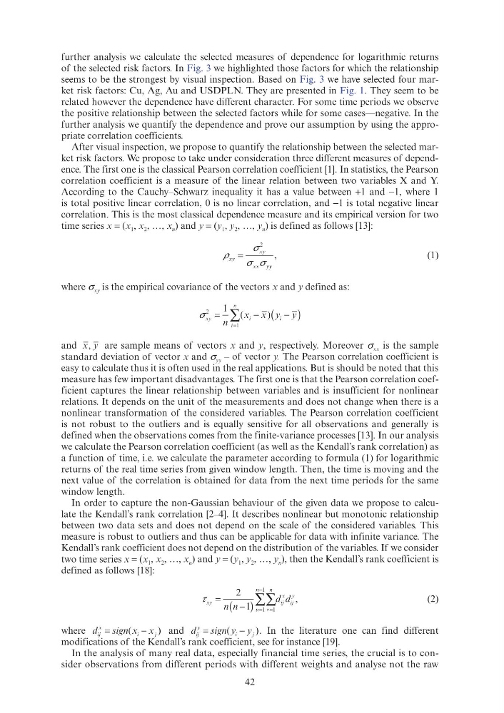
time series x = (x 1 , x 2 , …, x n ) and y = (y 1 , y 2 , …, y n ) is defined as follows [13]:
ρ
σ
σ σ
xy
xy
xx
σ σ yy
=
2
σ σ
,
(1)
where σ xy is the empirical covariance of the vectors x and y defined as:
σ xy
i
n
i
n
2
σ σ
1
1
=
(
)
i
y y
i
=
∑ (
)
i
x x
i
x
and x y are sample means of vectors x and y, respectively. Moreover σ xx is the sample
standard deviation of vector x and σ yy – of vector y. The Pearson correlation coefficient is
easy to calculate thus it is often used in the real applications. But is should be noted that this
measure has few important disadvantages. The first one is that the Pearson correlation coefficient captures the linear relationship between variables and is insufficient for nonlinear
relations. It depends on the unit of the measurements and does not change when there is a
nonlinear transformation of the considered variables. The Pearson correlation coefficient
is not robust to the outliers and is equally sensitive for all observations and generally is
defined when the observations comes from the finite-variance processes [13]. In our analysis
we calculate the Pearson correlation coefficient (as well as the Kendall’s rank correlation) as
a function of time, i.e. we calculate the parameter according to formula (1) for logarithmic
returns of the real time series from given window length. Then, the time is moving and the
next value of the correlation is obtained for data from the next time periods for the same
window length.
In order to capture the non-Gaussian behaviour of the given data we propose to calculate the Kendall’s rank correlation [2–4]. It describes nonlinear but monotonic relationship
between two data sets and does not depend on the scale of the considered variables. This
measure is robust to outliers and thus can be applicable for data with infinite variance. The
Kendall’s rank coefficient does not depend on the distribution of the variables. If we consider
two time series x = (x 1 , x 2 , …, x n ) and y = (y 1 , y 2 , …, y n ), then the Kendall’s rank coefficient is
defined as follows [18]:
τ xy
u
n
v
n
ij ij
y
n
d d
ij
x
i
= ( )
n − =
−
=
∑∑
2
1
1
1
,
(2)
where d
sign
ij
d d
i
j
sign(
)
x x
i
j
x
−
x
and d
sign y
ij
d d
i
j
y
sign(
)
y y
i
j
y
−
y
. In the literature one can find different
modifications of the Kendall’s rank coefficient, see for instance [19].
In the analysis of many real data, especially financial time series, the crucial is to consider observations from different periods with different weights and analyse not the raw
further analysis we calculate the selected measures of dependence for logarithmic returns
of the selected risk factors. In Fig. 3 we highlighted those factors for which the relationship
seems to be the strongest by visual inspection. Based on Fig. 3 we have selected four market risk factors: Cu, Ag, Au and USDPLN. They are presented in Fig. 1. They seem to be
related however the dependence have different character. For some time periods we observe
the positive relationship between the selected factors while for some cases—negative. In the
further analysis we quantify the dependence and prove our assumption by using the appropriate correlation coefficients.
After visual inspection, we propose to quantify the relationship between the selected market risk factors. We propose to take under consideration three different measures of dependence. The first one is the classical Pearson correlation coefficient [1]. In statistics, the Pearson
correlation coefficient is a measure of the linear relation between two variables X and Y.
According to the Cauchy–Schwarz inequality it has a value between +1 and −1, where 1
is total positive linear correlation, 0 is no linear correlation, and −1 is total negative linear
correlation. This is the most classical dependence measure and its empirical version for two
time series x = (x 1 , x 2 , …, x n ) and y = (y 1 , y 2 , …, y n ) is defined as follows [13]:
ρ
σ
σ σ
xy
xy
xx
σ σ yy
=
2
σ σ
,
(1)
where σ xy is the empirical covariance of the vectors x and y defined as:
σ xy
i
n
i
n
2
σ σ
1
1
=
(
)
i
y y
i
=
∑ (
)
i
x x
i
x
and x y are sample means of vectors x and y, respectively. Moreover σ xx is the sample
standard deviation of vector x and σ yy – of vector y. The Pearson correlation coefficient is
easy to calculate thus it is often used in the real applications. But is should be noted that this
measure has few important disadvantages. The first one is that the Pearson correlation coefficient captures the linear relationship between variables and is insufficient for nonlinear
relations. It depends on the unit of the measurements and does not change when there is a
nonlinear transformation of the considered variables. The Pearson correlation coefficient
is not robust to the outliers and is equally sensitive for all observations and generally is
defined when the observations comes from the finite-variance processes [13]. In our analysis
we calculate the Pearson correlation coefficient (as well as the Kendall’s rank correlation) as
a function of time, i.e. we calculate the parameter according to formula (1) for logarithmic
returns of the real time series from given window length. Then, the time is moving and the
next value of the correlation is obtained for data from the next time periods for the same
window length.
In order to capture the non-Gaussian behaviour of the given data we propose to calculate the Kendall’s rank correlation [2–4]. It describes nonlinear but monotonic relationship
between two data sets and does not depend on the scale of the considered variables. This
measure is robust to outliers and thus can be applicable for data with infinite variance. The
Kendall’s rank coefficient does not depend on the distribution of the variables. If we consider
two time series x = (x 1 , x 2 , …, x n ) and y = (y 1 , y 2 , …, y n ), then the Kendall’s rank coefficient is
defined as follows [18]:
τ xy
u
n
v
n
ij ij
y
n
d d
ij
x
i
= ( )
n − =
−
=
∑∑
2
1
1
1
,
(2)
where d
sign
ij
d d
i
j
sign(
)
x x
i
j
x
−
x
and d
sign y
ij
d d
i
j
y
sign(
)
y y
i
j
y
−
y
. In the literature one can find different
modifications of the Kendall’s rank coefficient, see for instance [19].
In the analysis of many real data, especially financial time series, the crucial is to consider observations from different periods with different weights and analyse not the raw