

553
For each indicator variable, 3 semi variograms were calculated, two in the XY plane (horizontal) and one with a 90° dip (vertical). All experimental semi variograms were performed
by a simple spherical structure
3 RESULTS AND DISCUSSIONS
3.1 Clustering
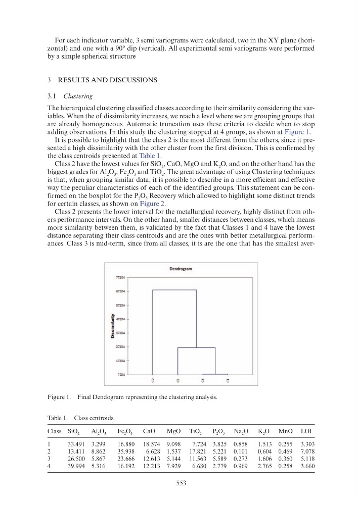
The hierarquical clustering classified classes according to their similarity considering the variables. When the of dissimilarity increases, we reach a level where we are grouping groups that
are already homogeneous. Automatic truncation uses these criteria to decide when to stop
adding observations. In this study the clustering stopped at 4 groups, as shown at Figure 1.
It is possible to highlight that the class 2 is the most different from the others, since it presented a high dissimilarity with the other cluster from the first division. This is confirmed by
the class centroids presented at Table 1.
Class 2 have the lowest values for SiO 2 , CaO, MgO and K 2 O, and on the other hand has the
biggest grades for Al 2 O 3 , Fe 2 O 3 and TiO 2 . The great advantage of using Clustering techniques
is that, when grouping similar data, it is possible to describe in a more efficient and effective
way the peculiar characteristics of each of the identified groups. This statement can be confirmed on the boxplot for the P 2 O 5 Recovery which allowed to highlight some distinct trends
for certain classes, as shown on Figure 2.
Class 2 presents the lower interval for the metallurgical recovery, highly distinct from others performance intervals. On the other hand, smaller distances between classes, which means
more similarity between them, is validated by the fact that Classes 1 and 4 have the lowest
distance separating their class centroids and are the ones with better metallurgical performances. Class 3 is mid-term, since from all classes, it is are the one that has the smallest averFigure 1. Final Dendogram representing the clustering analysis.
Table 1. Class centroids.
Class SiO 2
Al 2 O 3
Fe 2 O 3
CaO
MgO TiO 2
P 2 O 5 Na 2 O
K 2 O MnO LOI
1
33.491 3.299
16.880 18.574 9.098
7.724 3.825 0.858
1.513 0.255 3.303
2
13.411 8.862
35.938
6.628 1.537 17.821 5.221 0.101
0.604 0.469 7.078
3
26.500 5.867
23.666 12.613 5.144 11.563 5.589 0.273
1.606 0.360 5.118
4
39.994 5.316
16.192 12.213 7.929
6.680 2.779 0.969
2.765 0.258 3.660
Dendrogram
m04
67204
m04
f 47204
.E
·;;
Ql:l 37204
~
2n04
17204
7204
a