471
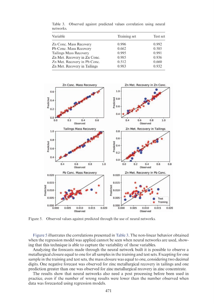
Figure 5 illustrates the correlations presented in Table 3. The non-linear behavior obtained
when the regression model was applied cannot be seen when neural networks are used, showing that this technique is able to capture the variability of those variables.
Analyzing the forecasts made through the neural network built it is possible to observe a
metallurgical closure equal to one for all samples in the training and test sets. Excepting for one
sample in the training and test sets, the mass closure was equal to one, considering two decimal
digits. One negative forecast was observed for zinc metallurgical recovery in tailings and one
prediction greater than one was observed for zinc metallurgical recovery in zinc concentrate.
The results show that neural networks also need a post processing before been used in
practice, even if the number of wrong results were lower than the number observed when
data was forecasted using regression models.
Table  3. Observed against predicted values correlation using neural
networks.
Variable
Training set
Test set
Zn Conc. Mass Recovery
0.996
0.992
Pb Conc. Mass Recovery
0.662
0.585
Tailings Mass Recovery
0.995
0.991
Zn Met. Recovery in Zn Conc.
0.985
0.936
Zn Met. Recovery in Pb Conc.
0.512
0.660
Zn Met. Recovery in Tailings
0.983
0.932
Figure 5. Observed values against predicted through the use of neural networks.
0.6
'0
~ 0 .4
'0
!'!
Q. 0 .2
0 .8
'0
~
'0
~ 0 .6
0.4
0.4
0.2
0.4
Observed
0.6
Observed
0 .8
0.6
1.0
0 . 020 .---- P _b _C_ o_ n_ c_. _M_a_s_s_R_e_c_o_v_e_ry'------,,
'0
0.015
~ 0 .010
i"
Q.
0.005
*
. . . . *
0.000 -1<"---~---~--~---1
0 .000
0.005
0. 010
Observed
0.015
0.020
'0
1.0
~ 0.8
'0
~ 0.6
0.4
0.8
0.6
'0
~ 0.4
'0
!'!
Q. 0.2
0.0
Zn Met. Recovery in Zn Cone.
0.4
0.6
0.8
1.0
Observed
Zn Met. Recovery in Ta ili ngs
0.0
0.2
0.4
Observed
*
0.6
0.8
0 . 020 .---z_n_M_e_t_. _R_e_c_o_v_e_:ry_ i n_P_b_C_ o_n_ c_. ~
0.015
*
~ 0.010
•
**
i"
*
Q.
*
0.005
•
•
Test
*
Training
0.000
0.000
0 .005
0.010
0.015
0.020
Observed