

449
method with the weighted sum method in terms of: (i) minimum maximum deviation between
ore and ore processing capacity per period, (ii) upper and lower maximum deviation between
copper fines and expected copper fines in the ore processing capacity per period, (iii) Overall
movement cost and time of shovel fleet, and finally (iv) resolution time. In the weighted sum
method, the weights u i assigned by the decision maker for each objective in decreasing order
take the values of 10,000; 100 and 10.
5 RESULTS AND DISCUSSION
In the case study, the weighted sum method needs 22.11 [h] to be carried out (resolution of
mMDP, mMDF, mD and WS(1,2,3)), while the hierarchical method needs 11.85 [h] (resolution of mMDP, mMDF(mMDP), mD(mMDP(mMDF)). Table 5 shows the results of the
mD, mMDP, and mMDF problems.
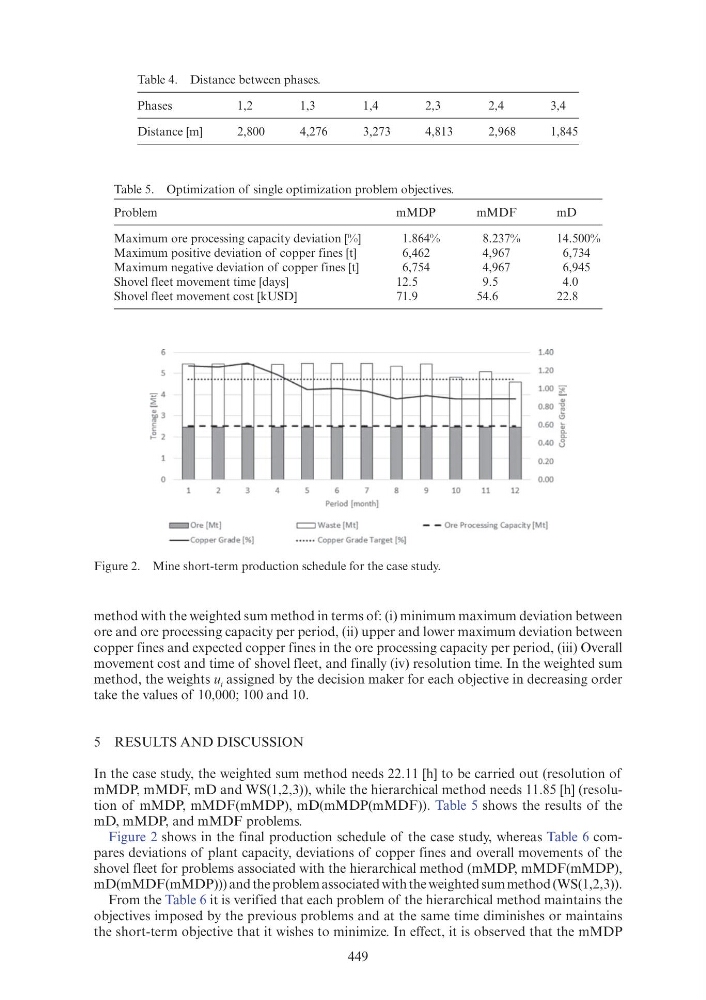
Figure 2 shows in the final production schedule of the case study, whereas Table 6 compares deviations of plant capacity, deviations of copper fines and overall movements of the
shovel fleet for problems associated with the hierarchical method (mMDP, mMDF(mMDP),
mD(mMDF(mMDP))) and the problem associated with the weighted sum method (WS(1,2,3)).
From the Table 6 it is verified that each problem of the hierarchical method maintains the
objectives imposed by the previous problems and at the same time diminishes or maintains
the short-term objective that it wishes to minimize. In effect, it is observed that the mMDP
Table 4. Distance between phases.
Phases
1,2
1,3
1,4
2,3
2,4
3,4
Distance [m]
2,800
4,276
3,273
4,813
2,968
1,845
Table 5. Optimization of single optimization problem objectives.
Problem
mMDP
mMDF
mD
Maximum ore processing capacity deviation [%]
1.864%
8.237%
14.500%
Maximum positive deviation of copper fines [t]
6,462
4,967
6,734
Maximum negative deviation of copper fines [t]
6,754
4,967
6,945
Shovel fleet movement time [days]
12.5
9.5
4.0
Shovel fleet movement cost [kUSD]
71.9
54.6
22.8
Figure 2. Mine short-term production schedule for the case study.
6
0
,..,_ ...... =!_..,......,.__........._,---- -
-
~
-
~
................ .... b:k ···························· ······· =····c:-:: ..... . . : . . . .
-~ - ~ -r- - ~ - r-- ~ - f.- -,...- - ~ -- - ~ - ,..._
-
,_
4
Period (month]
....
8
-
10
......
11
....
12
1.40
1.20
1.00 ~
~
0.80 -g
to
0.60 ~
0.40 8
0.20
0.00
=
ore(Mt]
- - Copper Grade(%(
=
waste(Mt]
- - Ore Processing Capacity [Mt]
•·• •·• Copper Grade Target(%]
method with the weighted sum method in terms of: (i) minimum maximum deviation between
ore and ore processing capacity per period, (ii) upper and lower maximum deviation between
copper fines and expected copper fines in the ore processing capacity per period, (iii) Overall
movement cost and time of shovel fleet, and finally (iv) resolution time. In the weighted sum
method, the weights u i assigned by the decision maker for each objective in decreasing order
take the values of 10,000; 100 and 10.
5 RESULTS AND DISCUSSION
In the case study, the weighted sum method needs 22.11 [h] to be carried out (resolution of
mMDP, mMDF, mD and WS(1,2,3)), while the hierarchical method needs 11.85 [h] (resolution of mMDP, mMDF(mMDP), mD(mMDP(mMDF)). Table 5 shows the results of the
mD, mMDP, and mMDF problems.
Figure 2 shows in the final production schedule of the case study, whereas Table 6 compares deviations of plant capacity, deviations of copper fines and overall movements of the
shovel fleet for problems associated with the hierarchical method (mMDP, mMDF(mMDP),
mD(mMDF(mMDP))) and the problem associated with the weighted sum method (WS(1,2,3)).
From the Table 6 it is verified that each problem of the hierarchical method maintains the
objectives imposed by the previous problems and at the same time diminishes or maintains
the short-term objective that it wishes to minimize. In effect, it is observed that the mMDP
Table 4. Distance between phases.
Phases
1,2
1,3
1,4
2,3
2,4
3,4
Distance [m]
2,800
4,276
3,273
4,813
2,968
1,845
Table 5. Optimization of single optimization problem objectives.
Problem
mMDP
mMDF
mD
Maximum ore processing capacity deviation [%]
1.864%
8.237%
14.500%
Maximum positive deviation of copper fines [t]
6,462
4,967
6,734
Maximum negative deviation of copper fines [t]
6,754
4,967
6,945
Shovel fleet movement time [days]
12.5
9.5
4.0
Shovel fleet movement cost [kUSD]
71.9
54.6
22.8
Figure 2. Mine short-term production schedule for the case study.
6
0
,..,_ ...... =!_..,......,.__........._,---- -
-
~
-
~
................ .... b:k ···························· ······· =····c:-:: ..... . . : . . . .
-~ - ~ -r- - ~ - r-- ~ - f.- -,...- - ~ -- - ~ - ,..._
-
,_
4
Period (month]
....
8
-
10
......
11
....
12
1.40
1.20
1.00 ~
~
0.80 -g
to
0.60 ~
0.40 8
0.20
0.00
=
ore(Mt]
- - Copper Grade(%(
=
waste(Mt]
- - Ore Processing Capacity [Mt]
•·• •·• Copper Grade Target(%]