

424
Then the model for crew assignment is defined by the objective function (12) subject to
Constraints (13), (14), (15) and (16).
If we consider as a set of nodes containing all pairs (v,k), and construct an arc between
nodes (v,k) and (vv,kk) if comp v,k,vv,kk,b = 1 for any base b, then the model can be seen as a flow
problem in this graph, similar to several crew scheduling and rostering models found in bibliography, for example.
4 NUMERICAL EXAMPLE
In this section, we present a numerical instance of a real case, transporting mineral products
and supplies between mines and several places (other mines, plants, ports, etc.). The case
includes a set of trains running for a 7-days period, say Monday to Sunday. Each train is
represented by a code, as follow:
T =
−
−
−
−
−
−
1203 1204 1220 1221 1250 1253 1701 1702 1703 1706
1709 1714 1711 1 1 1712
201 206
207 202
208 205
209 210
213 214
241 240
243 242
−
−
1712
201
−
−
202
208
−
−
210
213
−
−
240
243
S1101 1 1
1
2
1201
101
1
2
EMEL
EPAMPA
A
S
2
S
DISPAA I I
S
DISPCC I I
⎧
⎨
⎪
⎧ ⎧
⎪
⎪ ⎪
⎪
⎨ ⎨
⎪ ⎪
⎩
⎪ ⎪
⎨ ⎨ ⎨ ⎨
⎪
⎪ ⎪ ⎪ ⎪
⎪ ⎩ ⎩
⎪ ⎪
⎫
⎬
⎪
⎫ ⎫
⎪
⎪ ⎪
⎪
⎬ ⎬
⎪ ⎪
⎭
⎪
⎬ ⎬
⎪
⎪ ⎪
⎪ ⎭ ⎭
⎪ ⎪
For every train t T , the set K t has at least 80 elements (the possible locations for crew
replacements), value JE t
E is set at value 12 hours or 10.5 hours, depending of t. We only consider cyclical trains, that is to say, T T c
T T , and every train operate seven days. Moreover, there
are 5 camp bases where crews can stay for the 10-hours rest time:
B = {
}
CAMPCMZ CALAMA CAMPMEL OLLAGU PNORTE
CALAMA
OLLAGU
The maximal travel time admitted for transportation of crews between bases and locations for replacements is TE = 2 5
. hours. There are 3 operation zones, Z 1 ,Z 2 and Z 3 , and 2
zones for changes in common areas Zc Z Z
1
1
Z Z
2
Z
= ∩ and Zc Z Z
2
2
Z
3
Z Z
= ∩ . We test the model
for the number of crews M = 92,93 and 94, knowing that for M ≤ 91 the problem turns
infeasible.
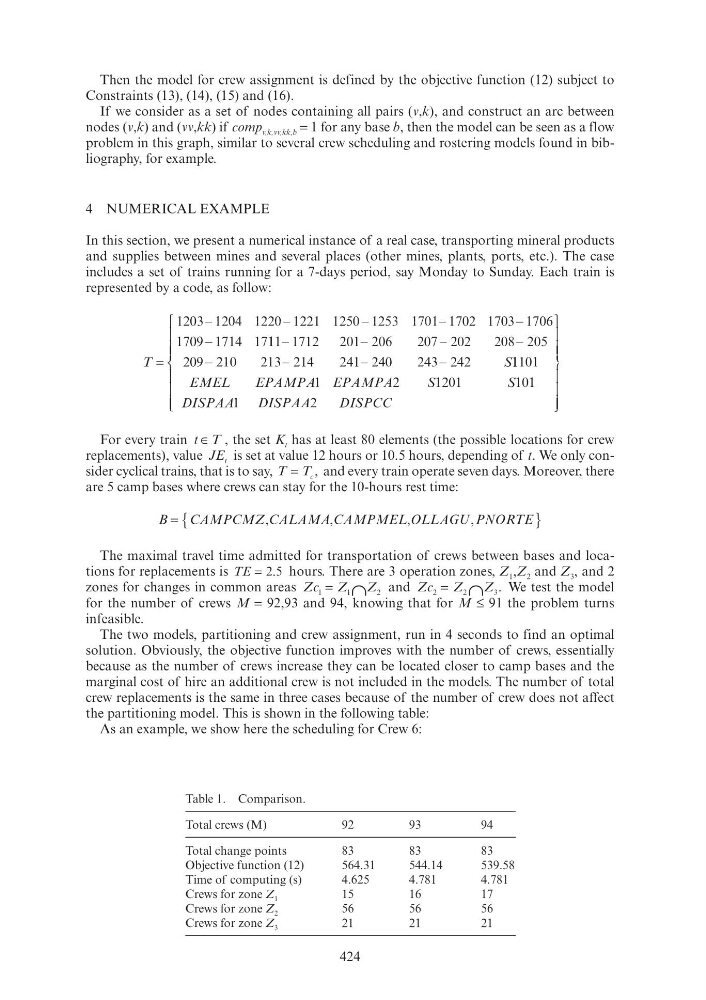
The two models, partitioning and crew assignment, run in 4 seconds to find an optimal
solution. Obviously, the objective function improves with the number of crews, essentially
because as the number of crews increase they can be located closer to camp bases and the
marginal cost of hire an additional crew is not included in the models. The number of total
crew replacements is the same in three cases because of the number of crew does not affect
the partitioning model. This is shown in the following table:
As an example, we show here the scheduling for Crew 6:
Table 1. Comparison.
Total crews (M)
92
93
94
Total change points
83
83
83
Objective function (12)
564.31
544.14
539.58
Time of computing (s)
4.625
4.781
4.781
Crews for zone Z 1
15
16
17
Crews for zone Z 2
56
56
56
Crews for zone Z 3
21
21
21
Then the model for crew assignment is defined by the objective function (12) subject to
Constraints (13), (14), (15) and (16).
If we consider as a set of nodes containing all pairs (v,k), and construct an arc between
nodes (v,k) and (vv,kk) if comp v,k,vv,kk,b = 1 for any base b, then the model can be seen as a flow
problem in this graph, similar to several crew scheduling and rostering models found in bibliography, for example.
4 NUMERICAL EXAMPLE
In this section, we present a numerical instance of a real case, transporting mineral products
and supplies between mines and several places (other mines, plants, ports, etc.). The case
includes a set of trains running for a 7-days period, say Monday to Sunday. Each train is
represented by a code, as follow:
T =
−
−
−
−
−
−
1203 1204 1220 1221 1250 1253 1701 1702 1703 1706
1709 1714 1711 1 1 1712
201 206
207 202
208 205
209 210
213 214
241 240
243 242
−
−
1712
201
−
−
202
208
−
−
210
213
−
−
240
243
S1101 1 1
1
2
1201
101
1
2
EMEL
EPAMPA
A
S
2
S
DISPAA I I
S
DISPCC I I
⎧
⎨
⎪
⎧ ⎧
⎪
⎪ ⎪
⎪
⎨ ⎨
⎪ ⎪
⎩
⎪ ⎪
⎨ ⎨ ⎨ ⎨
⎪
⎪ ⎪ ⎪ ⎪
⎪ ⎩ ⎩
⎪ ⎪
⎫
⎬
⎪
⎫ ⎫
⎪
⎪ ⎪
⎪
⎬ ⎬
⎪ ⎪
⎭
⎪
⎬ ⎬
⎪
⎪ ⎪
⎪ ⎭ ⎭
⎪ ⎪
For every train t T , the set K t has at least 80 elements (the possible locations for crew
replacements), value JE t
E is set at value 12 hours or 10.5 hours, depending of t. We only consider cyclical trains, that is to say, T T c
T T , and every train operate seven days. Moreover, there
are 5 camp bases where crews can stay for the 10-hours rest time:
B = {
}
CAMPCMZ CALAMA CAMPMEL OLLAGU PNORTE
CALAMA
OLLAGU
The maximal travel time admitted for transportation of crews between bases and locations for replacements is TE = 2 5
. hours. There are 3 operation zones, Z 1 ,Z 2 and Z 3 , and 2
zones for changes in common areas Zc Z Z
1
1
Z Z
2
Z
= ∩ and Zc Z Z
2
2
Z
3
Z Z
= ∩ . We test the model
for the number of crews M = 92,93 and 94, knowing that for M ≤ 91 the problem turns
infeasible.
The two models, partitioning and crew assignment, run in 4 seconds to find an optimal
solution. Obviously, the objective function improves with the number of crews, essentially
because as the number of crews increase they can be located closer to camp bases and the
marginal cost of hire an additional crew is not included in the models. The number of total
crew replacements is the same in three cases because of the number of crew does not affect
the partitioning model. This is shown in the following table:
As an example, we show here the scheduling for Crew 6:
Table 1. Comparison.
Total crews (M)
92
93
94
Total change points
83
83
83
Objective function (12)
564.31
544.14
539.58
Time of computing (s)
4.625
4.781
4.781
Crews for zone Z 1
15
16
17
Crews for zone Z 2
56
56
56
Crews for zone Z 3
21
21
21