

390
To model the conditional constraints (if constraints) an upper bound M is used, as
explained in Taha (2017) and AIMMS (2018), also known as big-M constraint type. This
can be seen in the constraint pair formed by (2) and (3) and also in constraints (10), (13),
and (14).
Constraints (2), (3) and (4) define and limit pp ih
*
to 0 if production activity of task i
happens after F, to F x ij otherwise and to p ih
* , since pp ih
*
is also the process period of
activity h
* .
Equation (5) guarantees that the starting date, x ij , will be greater than starting date constraint, r ij . (6) assures that only one machine will process a activity of a given task. (7) represents the flow of activities for each task.
Constraints (8), (9) and (10) models the relationship between different tasks in parallel
machines: if two tasks are processed by the same machine one has to be before other.
Expression (11) models extra dependencies between tasks according to input given. (12),
(13) and (14) defines the variable x ijh .
2.2 Implementation
The scheduling model was implemented in Python 3.7 with use of Anaconda distribution.
The linear programming solver used is Google OR Tools.
The code was written in Jupyter Notebook environment. User interface is done through a
spreadsheet where input data can be inserted and output values can be represented as a Gantt
chart. A graphical user interface (GUI) was built using wxFormBuilder and then built into a
single.exe Windows application with Pyinstaller.
A spreadsheet contains inputs already listed in 2.1.1.
Output is also a spreadsheet that holds all variables results. With x ij values it is possible to
create a Gantt chart to validate the result.
3 CASE STUDY
An exercise was performed using data from an underground gold mine in Brazil. AngloGold
Ashanti Cuiabá mine is located in the city of Sabará, state of Minas Gerais, in the Southeast
part of Brazil. The mine has reached a depth of 1300 m and produces approximately 1.3
Mtpa.
A Cuiabá monthly plan averages 25 tasks and 28 monitored activities. To simplify and generate an easier to understand example, a smaller part of a monthly plan was used considering
only 10 tasks and 5 activities.
Inputs were the same listed in Figure 5. Optimized scheduled was then compared to a
manual schedule done in advance considering task prioritization according to (production)/
(total duration) ratio.
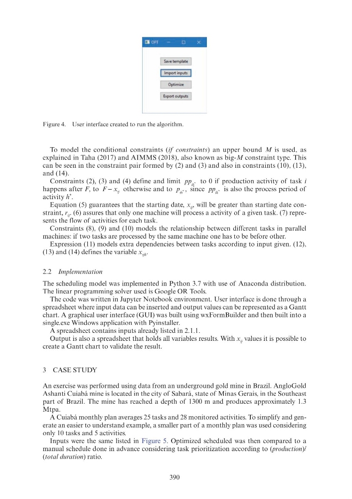
Figure 4. User interface created to run the algorithm.
Cli OPT
-
0
X
Sav~ t~mplat~
I Import inputs I
[
Optimize: --.J
[ Export out~
To model the conditional constraints (if constraints) an upper bound M is used, as
explained in Taha (2017) and AIMMS (2018), also known as big-M constraint type. This
can be seen in the constraint pair formed by (2) and (3) and also in constraints (10), (13),
and (14).
Constraints (2), (3) and (4) define and limit pp ih
*
to 0 if production activity of task i
happens after F, to F x ij otherwise and to p ih
* , since pp ih
*
is also the process period of
activity h
* .
Equation (5) guarantees that the starting date, x ij , will be greater than starting date constraint, r ij . (6) assures that only one machine will process a activity of a given task. (7) represents the flow of activities for each task.
Constraints (8), (9) and (10) models the relationship between different tasks in parallel
machines: if two tasks are processed by the same machine one has to be before other.
Expression (11) models extra dependencies between tasks according to input given. (12),
(13) and (14) defines the variable x ijh .
2.2 Implementation
The scheduling model was implemented in Python 3.7 with use of Anaconda distribution.
The linear programming solver used is Google OR Tools.
The code was written in Jupyter Notebook environment. User interface is done through a
spreadsheet where input data can be inserted and output values can be represented as a Gantt
chart. A graphical user interface (GUI) was built using wxFormBuilder and then built into a
single.exe Windows application with Pyinstaller.
A spreadsheet contains inputs already listed in 2.1.1.
Output is also a spreadsheet that holds all variables results. With x ij values it is possible to
create a Gantt chart to validate the result.
3 CASE STUDY
An exercise was performed using data from an underground gold mine in Brazil. AngloGold
Ashanti Cuiabá mine is located in the city of Sabará, state of Minas Gerais, in the Southeast
part of Brazil. The mine has reached a depth of 1300 m and produces approximately 1.3
Mtpa.
A Cuiabá monthly plan averages 25 tasks and 28 monitored activities. To simplify and generate an easier to understand example, a smaller part of a monthly plan was used considering
only 10 tasks and 5 activities.
Inputs were the same listed in Figure 5. Optimized scheduled was then compared to a
manual schedule done in advance considering task prioritization according to (production)/
(total duration) ratio.
Figure 4. User interface created to run the algorithm.
Cli OPT
-
0
X
Sav~ t~mplat~
I Import inputs I
[
Optimize: --.J
[ Export out~