

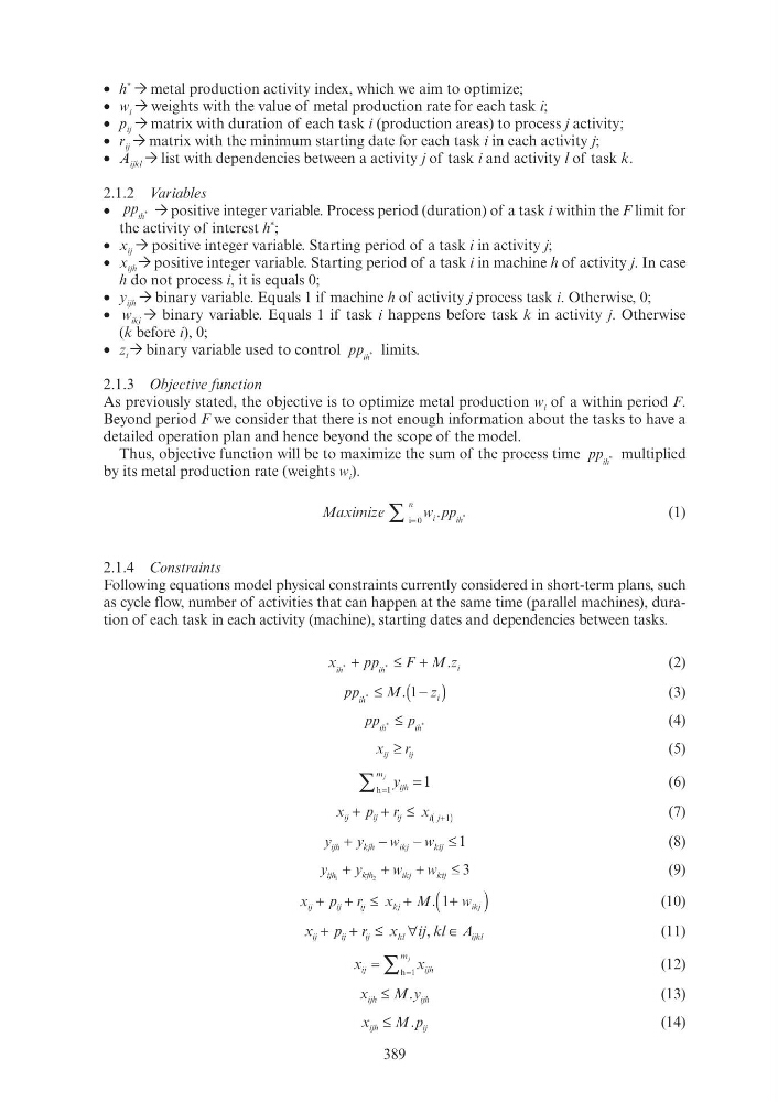
389
• h
*
metal production activity index, which we aim to optimize;
• w i weights with the value of metal production rate for each task i;
• p ij matrix with duration of each task i (production areas) to process j activity;
• r ij matrix with the minimum starting date for each task i in each activity j;
• A ijkl list with dependencies between a activity j of task i and activity l of task k.
2.1.2 Variables
• pp ih
*
positive integer variable. Process period (duration) of a task i within the F limit for
the activity of interest h
*
;
• x ij positive integer variable. Starting period of a task i in activity j;
• x ijh positive integer variable. Starting period of a task i in machine h of activity j. In case
h do not process i, it is equals 0;
• y ijh binary variable. Equals 1 if machine h of activity j process task i. Otherwise, 0;
• w ikj k
binary variable. Equals 1 if task i happens before task k in activity j. Otherwise
(k before i), 0;
• z i binary variable used to control pp ih
* limits.
2.1.3 Objective function
As previously stated, the objective is to optimize metal production w i of a within period F.
Beyond period F we consider that there is not enough information about the tasks to have a
detailed operation plan and hence beyond the scope of the model.
Thus, objective function will be to maximize the sum of the process time
ih
* multiplied
by its metal production rate (weights w i ).
Maximize
w pp
i
ih
n
. *
i=
∑ 0
(1)
2.1.4 Constraints
Following equations model physical constraints currently considered in short-term plans, such
as cycle flow, number of activities that can happen at the same time (parallel machines), duration of each task in each activity (machine), starting dates and dependencies between tasks.
x
pp
F
p p
M z
ih
ih
i
pp p
.
+ pp p pp p
+
(2)
pp
M
ih
*
.
≤ M ( )
z i
(3)
pp
p
ih
ih
*
*
p h
≤
(4)
x r
ij
ij
r r
≥
(5)
y ijh
m j
=
=
∑
1
1
h
(6)
x p r x
ij
ij
ij
r r
i
+ +
p ij
≤ ( )
j+
(7)
y
y
w
w
ijh
kjh
i
w
j j
kj
i i
kij i
+
−
y kjh j
−
≤
w kij i 1
(8)
y
y
w
w
ijh
kjh
i
w
j
kj
i i
kij i
1
2
y
h
kjh h
j j
3
+
+
y kjh j
+
≤
w kij i
(9)
x p r x
M
w
ij
ij
ij
r r
kj
ikj k
+ +
p ij
≤
+
x kj
(
)
1
. (
(10)
x p r x ij kl A
ij
ij
ij
r r
kl
ijk
A l
+ +
p ij
≤
∀
x kl
∈
,
(11)
x
x
ij
ijh
m j
∑ h 1
=
(12)
x
M y
ijh
ijh
.
(13)
x
M p
ijh
ij
.
(14)
• h
*
metal production activity index, which we aim to optimize;
• w i weights with the value of metal production rate for each task i;
• p ij matrix with duration of each task i (production areas) to process j activity;
• r ij matrix with the minimum starting date for each task i in each activity j;
• A ijkl list with dependencies between a activity j of task i and activity l of task k.
2.1.2 Variables
• pp ih
*
positive integer variable. Process period (duration) of a task i within the F limit for
the activity of interest h
*
;
• x ij positive integer variable. Starting period of a task i in activity j;
• x ijh positive integer variable. Starting period of a task i in machine h of activity j. In case
h do not process i, it is equals 0;
• y ijh binary variable. Equals 1 if machine h of activity j process task i. Otherwise, 0;
• w ikj k
binary variable. Equals 1 if task i happens before task k in activity j. Otherwise
(k before i), 0;
• z i binary variable used to control pp ih
* limits.
2.1.3 Objective function
As previously stated, the objective is to optimize metal production w i of a within period F.
Beyond period F we consider that there is not enough information about the tasks to have a
detailed operation plan and hence beyond the scope of the model.
Thus, objective function will be to maximize the sum of the process time
ih
* multiplied
by its metal production rate (weights w i ).
Maximize
w pp
i
ih
n
. *
i=
∑ 0
(1)
2.1.4 Constraints
Following equations model physical constraints currently considered in short-term plans, such
as cycle flow, number of activities that can happen at the same time (parallel machines), duration of each task in each activity (machine), starting dates and dependencies between tasks.
x
pp
F
p p
M z
ih
ih
i
pp p
.
+ pp p pp p
+
(2)
pp
M
ih
*
.
≤ M ( )
z i
(3)
pp
p
ih
ih
*
*
p h
≤
(4)
x r
ij
ij
r r
≥
(5)
y ijh
m j
=
=
∑
1
1
h
(6)
x p r x
ij
ij
ij
r r
i
+ +
p ij
≤ ( )
j+
(7)
y
y
w
w
ijh
kjh
i
w
j j
kj
i i
kij i
+
−
y kjh j
−
≤
w kij i 1
(8)
y
y
w
w
ijh
kjh
i
w
j
kj
i i
kij i
1
2
y
h
kjh h
j j
3
+
+
y kjh j
+
≤
w kij i
(9)
x p r x
M
w
ij
ij
ij
r r
kj
ikj k
+ +
p ij
≤
+
x kj
(
)
1
. (
(10)
x p r x ij kl A
ij
ij
ij
r r
kl
ijk
A l
+ +
p ij
≤
∀
x kl
∈
,
(11)
x
x
ij
ijh
m j
∑ h 1
=
(12)
x
M y
ijh
ijh
.
(13)
x
M p
ijh
ij
.
(14)