

316
normalized units, the area under the ROC curve (henceforth, AUC) is equal to the probability
that a classifier will rank a randomly chosen positive instance higher than a randomly chosen
negative one. Since a perfect classifier has an area equal to 1, this means, in praxis, that the
AUC informs us about the quality of the classifier: How near is our model from achieving a
perfect classification. This is shown in Table 2.
b. Confusion Matrix:
Let us consider a set of pillars that can be separated in terms of the existence or inexistence of
damage due to collapse processes. This is a situation for which the output is binary and mutually exclusive, where the presence of damage is considered a “success” and “failure” when otherwise. Thus there are four possible results for such a problem. If the output value is a success
while the evaluated instance is also a success (this is, an output value labeling a pillar as damaged when it actually is), then it is called a True Positive (TP). On the other hand, if the output a
failure while the evaluated instance is also a failure (this is, an output value that labels a pillar as
undamaged when the same pillar is actually undamaged), then it is called a True Negative (TN).
The misclassifications of the model are called False Positives (FP) when the evaluated
instance is a failure while the output is labeled as a success (this is, classifying a pillar as damaged when it is actually undamaged), and False Negatives (FN) when the evaluated instance
is a success while the output is labeled as a failure (this is, classifying a pillar as undamaged
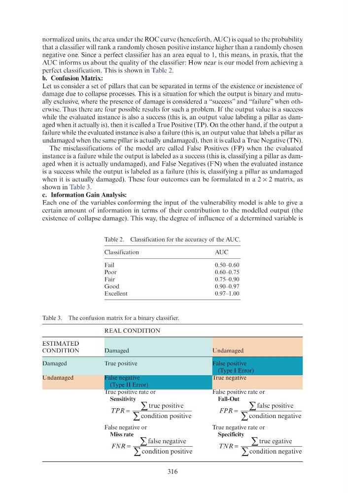
when it is actually damaged). These four outcomes can be formulated in a 2 × 2 matrix, as
shown in Table 3.
c. Information Gain Analysis:
Each one of the variables conforming the input of the vulnerability model is able to give a
certain amount of information in terms of their contribution to the modelled output (the
existence of collapse damage). This way, the degree of influence of a determined variable is
Table 2. Classification for the accuracy of the AUC.
Classification
AUC
Fail
0.50–0.60
Poor
0.60–0.75
Fair
0.75–0.90
Good
0.90–0.97
Excellent
0.97–1.00
Table 3. The confusion matrix for a binary classifier.
REAL CONDITION
ESTIMATED
CONDITION
Damaged
Undamaged
Damaged
True positive
False positive
(Type I Error)
Undamaged
False negative
(Type II Error)
True negative
True positive rate or
Sensitivity
TPR =
∑
∑
true positive
condition positive
False positive rate or
Fall-Out
FPR =
∑
∑
false positive
condition negative
False negative or
Miss rate
FNR N N =
∑
∑
false negative
condition positive
True negative rate or
Specificity
TNR N N =
∑
∑
true egative
condition negative
normalized units, the area under the ROC curve (henceforth, AUC) is equal to the probability
that a classifier will rank a randomly chosen positive instance higher than a randomly chosen
negative one. Since a perfect classifier has an area equal to 1, this means, in praxis, that the
AUC informs us about the quality of the classifier: How near is our model from achieving a
perfect classification. This is shown in Table 2.
b. Confusion Matrix:
Let us consider a set of pillars that can be separated in terms of the existence or inexistence of
damage due to collapse processes. This is a situation for which the output is binary and mutually exclusive, where the presence of damage is considered a “success” and “failure” when otherwise. Thus there are four possible results for such a problem. If the output value is a success
while the evaluated instance is also a success (this is, an output value labeling a pillar as damaged when it actually is), then it is called a True Positive (TP). On the other hand, if the output a
failure while the evaluated instance is also a failure (this is, an output value that labels a pillar as
undamaged when the same pillar is actually undamaged), then it is called a True Negative (TN).
The misclassifications of the model are called False Positives (FP) when the evaluated
instance is a failure while the output is labeled as a success (this is, classifying a pillar as damaged when it is actually undamaged), and False Negatives (FN) when the evaluated instance
is a success while the output is labeled as a failure (this is, classifying a pillar as undamaged
when it is actually damaged). These four outcomes can be formulated in a 2 × 2 matrix, as
shown in Table 3.
c. Information Gain Analysis:
Each one of the variables conforming the input of the vulnerability model is able to give a
certain amount of information in terms of their contribution to the modelled output (the
existence of collapse damage). This way, the degree of influence of a determined variable is
Table 2. Classification for the accuracy of the AUC.
Classification
AUC
Fail
0.50–0.60
Poor
0.60–0.75
Fair
0.75–0.90
Good
0.90–0.97
Excellent
0.97–1.00
Table 3. The confusion matrix for a binary classifier.
REAL CONDITION
ESTIMATED
CONDITION
Damaged
Undamaged
Damaged
True positive
False positive
(Type I Error)
Undamaged
False negative
(Type II Error)
True negative
True positive rate or
Sensitivity
TPR =
∑
∑
true positive
condition positive
False positive rate or
Fall-Out
FPR =
∑
∑
false positive
condition negative
False negative or
Miss rate
FNR N N =
∑
∑
false negative
condition positive
True negative rate or
Specificity
TNR N N =
∑
∑
true egative
condition negative