

315
where b jm is the predicted value in the region R jm . Then, the coefficients b jm are multiplied by
some value λ m , chosen to minimize the loss function, which allows us to update the model at
each iteration as shown in Equations 6 and 7:
F
F
h
m
F F
m
F F
m m
h
( )
x x =
( )
x +
( )
x
−1
λ m
(6)
λ
λ
λ
m
λ λ
x R
i
m
m
λ
i
j
R m
j j
y i m
h
λ m m
λ
( )
i
( )
i
x
(
)
⎡
⎣
⎢
⎡ ⎡
⎢ ⎣ ⎣
⎢ ⎢
⎤
⎦
⎥
⎤ ⎤
⎥ ⎦ ⎦
⎥ ⎥
−
∑
g
L
1
(7)
Notice that this kind of method corresponds to a heuristic procedure and, by extension,
does not generate exact analytical solutions or values for the desired problem, but approximations to such values (in case they exist).
5.2 Training, validation and application sets
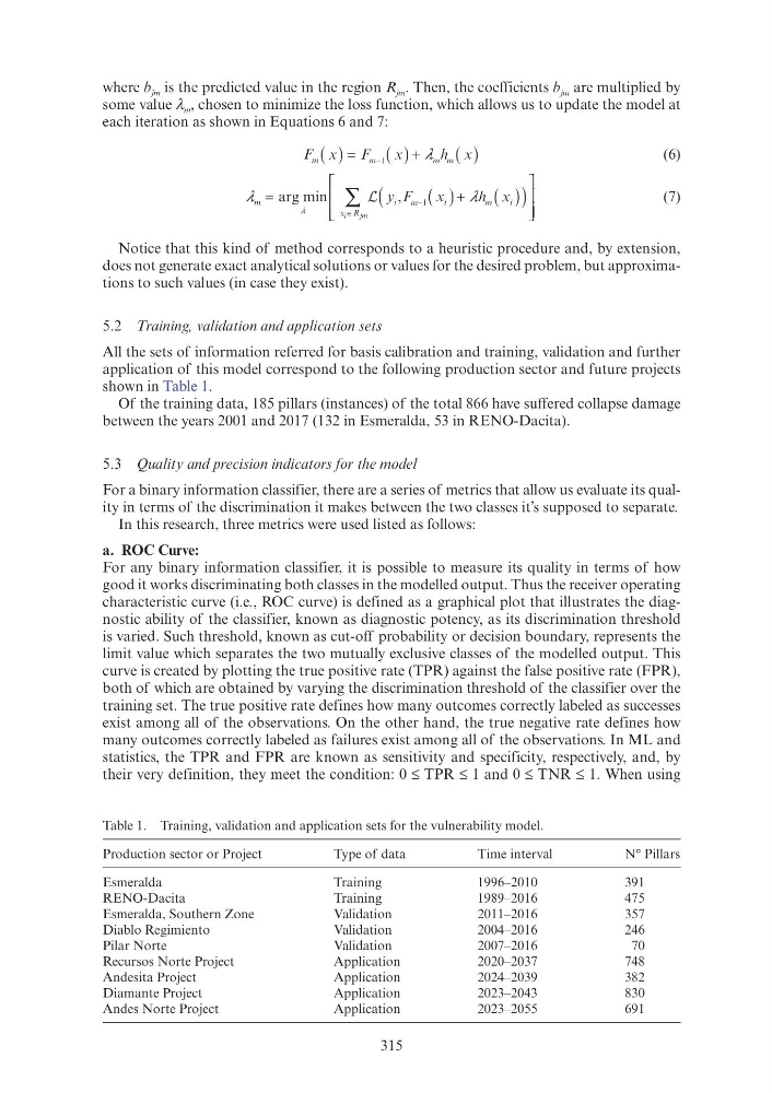
All the sets of information referred for basis calibration and training, validation and further
application of this model correspond to the following production sector and future projects
shown in Table 1.
Of the training data, 185 pillars (instances) of the total 866 have suffered collapse damage
between the years 2001 and 2017 (132 in Esmeralda, 53 in RENO-Dacita).
5.3 Quality and precision indicators for the model
For a binary information classifier, there are a series of metrics that allow us evaluate its quality in terms of the discrimination it makes between the two classes it’s supposed to separate.
In this research, three metrics were used listed as follows:
a. ROC Curve:
For any binary information classifier, it is possible to measure its quality in terms of how
good it works discriminating both classes in the modelled output. Thus the receiver operating
characteristic curve (i.e., ROC curve) is defined as a graphical plot that illustrates the diagnostic ability of the classifier, known as diagnostic potency, as its discrimination threshold
is varied. Such threshold, known as cut-off probability or decision boundary, represents the
limit value which separates the two mutually exclusive classes of the modelled output. This
curve is created by plotting the true positive rate (TPR) against the false positive rate (FPR),
both of which are obtained by varying the discrimination threshold of the classifier over the
training set. The true positive rate defines how many outcomes correctly labeled as successes
exist among all of the observations. On the other hand, the true negative rate defines how
many outcomes correctly labeled as failures exist among all of the observations. In ML and
statistics, the TPR and FPR are known as sensitivity and specificity, respectively, and, by
their very definition, they meet the condition: 0 ≤ TPR ≤ 1 and 0 ≤ TNR ≤ 1. When using
Table 1. Training, validation and application sets for the vulnerability model.
Production sector or Project
Type of data
Time interval
N° Pillars
Esmeralda
Training
1996–2010
391
RENO-Dacita
Training
1989–2016
475
Esmeralda, Southern Zone
Validation
2011–2016
357
Diablo Regimiento
Validation
2004–2016
246
Pilar Norte
Validation
2007–2016
70
Recursos Norte Project
Application
2020–2037
748
Andesita Project
Application
2024–2039
382
Diamante Project
Application
2023–2043
830
Andes Norte Project
Application
2023–2055
691
where b jm is the predicted value in the region R jm . Then, the coefficients b jm are multiplied by
some value λ m , chosen to minimize the loss function, which allows us to update the model at
each iteration as shown in Equations 6 and 7:
F
F
h
m
F F
m
F F
m m
h
( )
x x =
( )
x +
( )
x
−1
λ m
(6)
λ
λ
λ
m
λ λ
x R
i
m
m
λ
i
j
R m
j j
y i m
h
λ m m
λ
( )
i
( )
i
x
(
)
⎡
⎣
⎢
⎡ ⎡
⎢ ⎣ ⎣
⎢ ⎢
⎤
⎦
⎥
⎤ ⎤
⎥ ⎦ ⎦
⎥ ⎥
−
∑
g
L
1
(7)
Notice that this kind of method corresponds to a heuristic procedure and, by extension,
does not generate exact analytical solutions or values for the desired problem, but approximations to such values (in case they exist).
5.2 Training, validation and application sets
All the sets of information referred for basis calibration and training, validation and further
application of this model correspond to the following production sector and future projects
shown in Table 1.
Of the training data, 185 pillars (instances) of the total 866 have suffered collapse damage
between the years 2001 and 2017 (132 in Esmeralda, 53 in RENO-Dacita).
5.3 Quality and precision indicators for the model
For a binary information classifier, there are a series of metrics that allow us evaluate its quality in terms of the discrimination it makes between the two classes it’s supposed to separate.
In this research, three metrics were used listed as follows:
a. ROC Curve:
For any binary information classifier, it is possible to measure its quality in terms of how
good it works discriminating both classes in the modelled output. Thus the receiver operating
characteristic curve (i.e., ROC curve) is defined as a graphical plot that illustrates the diagnostic ability of the classifier, known as diagnostic potency, as its discrimination threshold
is varied. Such threshold, known as cut-off probability or decision boundary, represents the
limit value which separates the two mutually exclusive classes of the modelled output. This
curve is created by plotting the true positive rate (TPR) against the false positive rate (FPR),
both of which are obtained by varying the discrimination threshold of the classifier over the
training set. The true positive rate defines how many outcomes correctly labeled as successes
exist among all of the observations. On the other hand, the true negative rate defines how
many outcomes correctly labeled as failures exist among all of the observations. In ML and
statistics, the TPR and FPR are known as sensitivity and specificity, respectively, and, by
their very definition, they meet the condition: 0 ≤ TPR ≤ 1 and 0 ≤ TNR ≤ 1. When using
Table 1. Training, validation and application sets for the vulnerability model.
Production sector or Project
Type of data
Time interval
N° Pillars
Esmeralda
Training
1996–2010
391
RENO-Dacita
Training
1989–2016
475
Esmeralda, Southern Zone
Validation
2011–2016
357
Diablo Regimiento
Validation
2004–2016
246
Pilar Norte
Validation
2007–2016
70
Recursos Norte Project
Application
2020–2037
748
Andesita Project
Application
2024–2039
382
Diamante Project
Application
2023–2043
830
Andes Norte Project
Application
2023–2055
691