

241
the covariance ˆ
12
C (0)
12
between the Gaussian variables Y 1 (x) and Y 2 (x) at the same point (h
equal to zero). This covariance can be estimated using the statistical correlation between Y 1
and Y 2,Mig (inexact samples migrated to neighboring exact data location for a short distance;
see Figure 1) and the variances of Y 1 (x) and Y 2 (x).
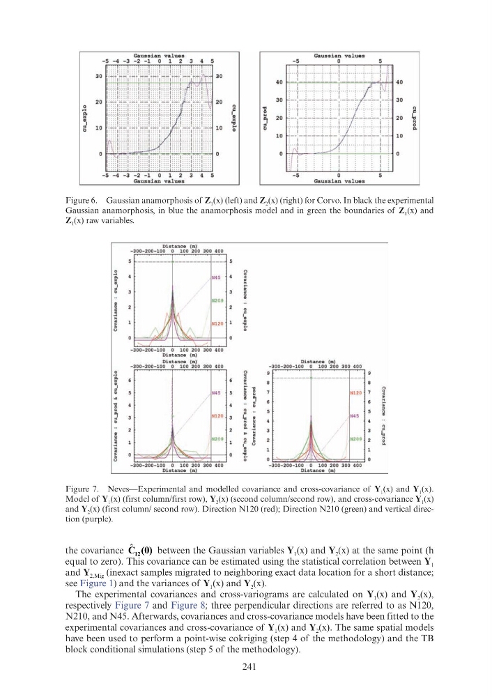
The experimental covariances and cross-variograms are calculated on Y 1 (x) and Y 2 (x),
respectively Figure 7 and Figure 8; three perpendicular directions are referred to as N120,
N210, and N45. Afterwards, covariances and cross-covariance models have been fitted to the
experimental covariances and cross-covariance of Y 1 (x) and Y 2 (x). The same spatial models
have been used to perform a point-wise cokriging (step 4 of the methodology) and the TB
block conditional simulations (step 5 of the methodology).
Figure 6. Gaussian anamorphosis of Z 1 (x) (left) and Z 2 (x) (right) for Corvo. In black the experimental
Gaussian anamorphosis, in blue the anamorphosis model and in green the boundaries of Z 1 (x) and
Z 1 (x) raw variables.
Figure 7. Neves—Experimental and modelled covariance and cross-covariance of Y 1 (x) and Y 1 (x).
Model of Y 1 (x) (first column/first row), Y 2 (x) (second column/second row), and cross-covariance Y 1 (x)
and Y 2 (x) (first column/ second row). Direction N120 (red); Direction N210 (green) and vertical direction (purple).
30
2 0
~
"'
"
. I
0
0
1 0
.
· ~
8
30
2 0
10
Dist ance {m)
-30 0 -200-100 0 10 0 200 3 00 40 0
. N45
N2 0 9
Di s t a n c fi (m)
Dista n c e (m)
-30 0-20 0 - 100 0 100 200 300 4 0 0
_.. N4 5
N12 0
N2 0 9
30 0 2 00 1 00 0 100 200 3 00 4 0 0
Dista nce (m)
0
, "
. "
'g.
0
n
0
~- ~
g ~
g
0
"
~
8.
0
"
I
. "
" ~
0
,
0
" '1 0 0
Gaussian values
0
4 0
30
20
1 0
Di s t ance (m)
- 300-200 - 1 00 0 1 00 20 0 3 00 400
9
N1 20 7
N45
4 0
3 0
0
2 0
"
1,
" 0
0.
10
the covariance ˆ
12
C (0)
12
between the Gaussian variables Y 1 (x) and Y 2 (x) at the same point (h
equal to zero). This covariance can be estimated using the statistical correlation between Y 1
and Y 2,Mig (inexact samples migrated to neighboring exact data location for a short distance;
see Figure 1) and the variances of Y 1 (x) and Y 2 (x).
The experimental covariances and cross-variograms are calculated on Y 1 (x) and Y 2 (x),
respectively Figure 7 and Figure 8; three perpendicular directions are referred to as N120,
N210, and N45. Afterwards, covariances and cross-covariance models have been fitted to the
experimental covariances and cross-covariance of Y 1 (x) and Y 2 (x). The same spatial models
have been used to perform a point-wise cokriging (step 4 of the methodology) and the TB
block conditional simulations (step 5 of the methodology).
Figure 6. Gaussian anamorphosis of Z 1 (x) (left) and Z 2 (x) (right) for Corvo. In black the experimental
Gaussian anamorphosis, in blue the anamorphosis model and in green the boundaries of Z 1 (x) and
Z 1 (x) raw variables.
Figure 7. Neves—Experimental and modelled covariance and cross-covariance of Y 1 (x) and Y 1 (x).
Model of Y 1 (x) (first column/first row), Y 2 (x) (second column/second row), and cross-covariance Y 1 (x)
and Y 2 (x) (first column/ second row). Direction N120 (red); Direction N210 (green) and vertical direction (purple).
30
2 0
~
"'
"
. I
0
0
1 0
.
· ~
8
30
2 0
10
Dist ance {m)
-30 0 -200-100 0 10 0 200 3 00 40 0
. N45
N2 0 9
Di s t a n c fi (m)
Dista n c e (m)
-30 0-20 0 - 100 0 100 200 300 4 0 0
_.. N4 5
N12 0
N2 0 9
30 0 2 00 1 00 0 100 200 3 00 4 0 0
Dista nce (m)
0
, "
. "
'g.
0
n
0
~- ~
g ~
g
0
"
~
8.
0
"
I
. "
" ~
0
,
0
" '1 0 0
Gaussian values
0
4 0
30
20
1 0
Di s t ance (m)
- 300-200 - 1 00 0 1 00 20 0 3 00 400
9
N1 20 7
N45
4 0
3 0
0
2 0
"
1,
" 0
0.
10