

240
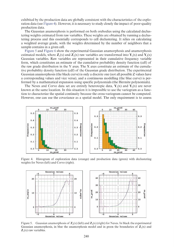
exhibited by the production data are globally consistent with the characteristics of the exploration data (see Figure 4). However, it is necessary to study closely the impact of poor-quality
production data.
The Gaussian anamorphosis is performed on both orebodies using the calculated declustering weights estimated from raw variables. These weights are obtained by running a declustering process and this essentially corresponds to cell declustering. It relies on calculating
a weighted average grade, with the weights determined by the number of neighbors that a
sample contains in a given cell.
Figure 5 and Figure 6 show the experimental Gaussian anamorphosis and anamorphosis
estimated models, where Z 1 (x) and Z 2 (x) raw variables are transformed into Y 1 (x) and Y 2 (x)
Gaussian variables. Raw variables are represented in their cumulative frequency variable
form, which constitutes an estimate of the cumulative probability density function (cdf) of
the raw grade distribution in the Y axes. The X axes constitute an estimate of the cumulative probability density function (cdf) of the Gaussian grade distribution. The experimental
Gaussian anamorphosis (the black curve) is only a discrete one (not all possible Z values have
a corresponding values and vice versa), and a continuous modelling (the blue curve) is performed by a mathematical expansion using specific polynomials (the Hermite polynomials).
The Neves and Corvo data set are entirely heterotopic data, Y 1 (x) and Y 2 (x) are never
known at the same location. In this situation it is impossible to use the variogram as a function to characterize the spatial continuity because the cross-variogram cannot be computed.
However, one can use the covariance as a spatial model. The only requirement is to assess
Figure 4. Histogram of exploration data (orange) and production data (green) with declustering
weights for Neves (left) and Corvo (right).
Figure 5. Gaussian anamorphosis of Z 1 (x) (left) and Z 2 (x) (right) for Neves. In black the experimental
Gaussian anamorphosis, in blue the anamorphosis model and in green the boundaries of Z 1 (x) and
Z 1 (x) raw variables.
0 . 5
0. 4
.
-~ tl 0. 3
" ~
~ 0. 2
..
0.1
20
~
"' "
10
w
o'
u
Gaussian va l ues
0
0. 5
0. 4 ..,
"
0.3 ~
~~
0. 2
0. 1
20
Q
10
"
I
. "
'g.
0
0. 3
.
-~ tl 0. 2
" ~
. "
..
"
0
"
"'
" u
0.1
40
30
20
10
Gaussian values
0
0. 3
..,
"
0.2 ~
~~
0.1
40
30
20
Q
~
" 0
0.
1 0
exhibited by the production data are globally consistent with the characteristics of the exploration data (see Figure 4). However, it is necessary to study closely the impact of poor-quality
production data.
The Gaussian anamorphosis is performed on both orebodies using the calculated declustering weights estimated from raw variables. These weights are obtained by running a declustering process and this essentially corresponds to cell declustering. It relies on calculating
a weighted average grade, with the weights determined by the number of neighbors that a
sample contains in a given cell.
Figure 5 and Figure 6 show the experimental Gaussian anamorphosis and anamorphosis
estimated models, where Z 1 (x) and Z 2 (x) raw variables are transformed into Y 1 (x) and Y 2 (x)
Gaussian variables. Raw variables are represented in their cumulative frequency variable
form, which constitutes an estimate of the cumulative probability density function (cdf) of
the raw grade distribution in the Y axes. The X axes constitute an estimate of the cumulative probability density function (cdf) of the Gaussian grade distribution. The experimental
Gaussian anamorphosis (the black curve) is only a discrete one (not all possible Z values have
a corresponding values and vice versa), and a continuous modelling (the blue curve) is performed by a mathematical expansion using specific polynomials (the Hermite polynomials).
The Neves and Corvo data set are entirely heterotopic data, Y 1 (x) and Y 2 (x) are never
known at the same location. In this situation it is impossible to use the variogram as a function to characterize the spatial continuity because the cross-variogram cannot be computed.
However, one can use the covariance as a spatial model. The only requirement is to assess
Figure 4. Histogram of exploration data (orange) and production data (green) with declustering
weights for Neves (left) and Corvo (right).
Figure 5. Gaussian anamorphosis of Z 1 (x) (left) and Z 2 (x) (right) for Neves. In black the experimental
Gaussian anamorphosis, in blue the anamorphosis model and in green the boundaries of Z 1 (x) and
Z 1 (x) raw variables.
0 . 5
0. 4
.
-~ tl 0. 3
" ~
~ 0. 2
..
0.1
20
~
"' "
10
w
o'
u
Gaussian va l ues
0
0. 5
0. 4 ..,
"
0.3 ~
~~
0. 2
0. 1
20
Q
10
"
I
. "
'g.
0
0. 3
.
-~ tl 0. 2
" ~
. "
..
"
0
"
"'
" u
0.1
40
30
20
10
Gaussian values
0
0. 3
..,
"
0.2 ~
~~
0.1
40
30
20
Q
~
" 0
0.
1 0