

239
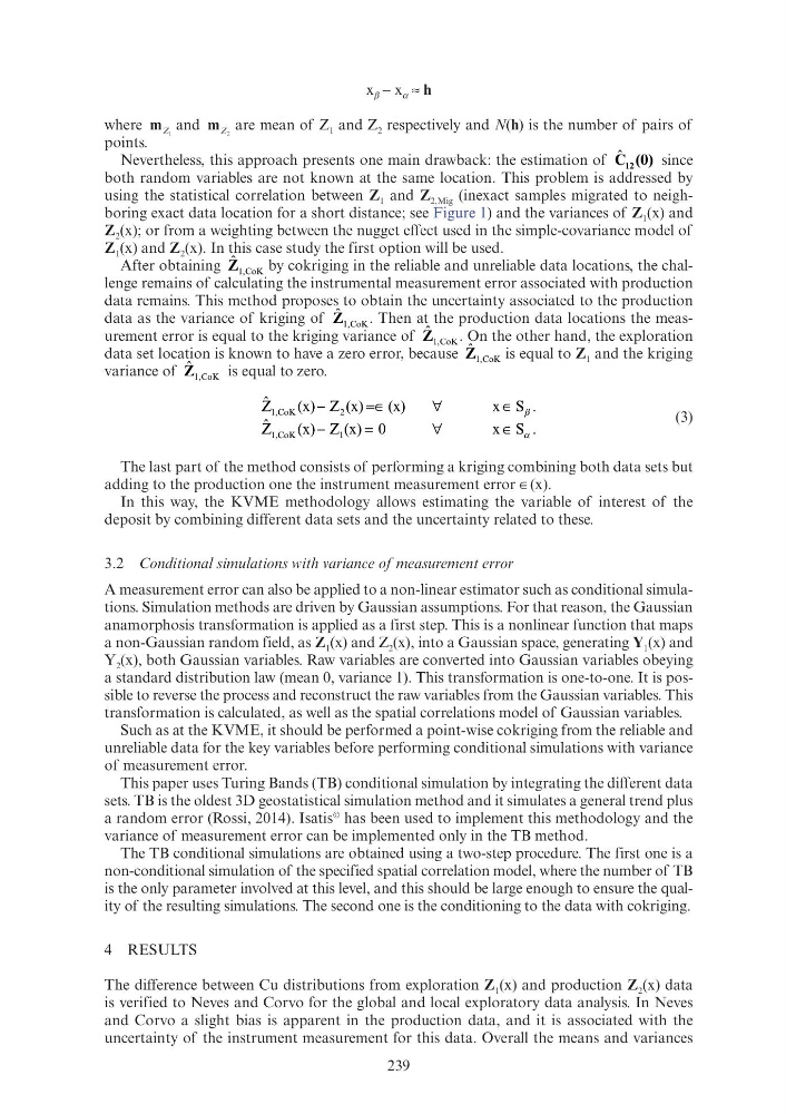
x β − x α ≈ h
where m Z 1
Z Z and m Z 2
Z are mean of Z 1 and Z 2 respectively and N(h) is the number of pairs of
points.
Nevertheless, this approach presents one main drawback: the estimation of ˆ
12
C (0)
12
since
both random variables are not known at the same location. This problem is addressed by
using the statistical correlation between Z 1 and Z 2,Mig (inexact samples migrated to neighboring exact data location for a short distance; see Figure 1) and the variances of Z 1 (x) and
Z 2 (x); or from a weighting between the nugget effect used in the simple-covariance model of
Z 1 (x) and Z 2 (x). In this case study the first option will be used.
After obtaining 1,CoK
ˆ
Z
by cokriging in the reliable and unreliable data locations, the challenge remains of calculating the instrumental measurement error associated with production
data remains. This method proposes to obtain the uncertainty associated to the production
data as the variance of kriging of 1,CoK
ˆ
Z
. Then at the production data locations the measurement error is equal to the kriging variance of 1,CoK
ˆ
Z
. On the other hand, the exploration
data set location is known to have a zero error, because 1,CoK
ˆ
Z
is equal to Z 1 and the kriging
variance of 1,CoK
ˆ
Z
is equal to zero.
1,CoK
2
1,CoK
1
ˆ
Z
(x) Z (x)
(x)
x S .
1,CoK
2
ˆ
Z
(x) Z (x) 0
x S .
1,CoK
1
β
α
Z (x)
(x)
x
Z (x)
(x)
x
2
Z (x) 0
x
Z (x) 0
x
1
(3)
The last part of the method consists of performing a kriging combining both data sets but
adding to the production one the instrument measurement error ∈(x).
In this way, the KVME methodology allows estimating the variable of interest of the
deposit by combining different data sets and the uncertainty related to these.
3.2 Conditional simulations with variance of measurement error
A measurement error can also be applied to a non-linear estimator such as conditional simulations. Simulation methods are driven by Gaussian assumptions. For that reason, the Gaussian
anamorphosis transformation is applied as a first step. This is a nonlinear function that maps
a non-Gaussian random field, as Z 1 (x) and Z 2 (x), into a Gaussian space, generating Y 1 (x) and
Y 2 (x), both Gaussian variables. Raw variables are converted into Gaussian variables obeying
a standard distribution law (mean 0, variance 1). This transformation is one-to-one. It is possible to reverse the process and reconstruct the raw variables from the Gaussian variables. This
transformation is calculated, as well as the spatial correlations model of Gaussian variables.
Such as at the KVME, it should be performed a point-wise cokriging from the reliable and
unreliable data for the key variables before performing conditional simulations with variance
of measurement error.
This paper uses Turing Bands (TB) conditional simulation by integrating the different data
sets. TB is the oldest 3D geostatistical simulation method and it simulates a general trend plus
a random error (Rossi, 2014). Isatis
© has been used to implement this methodology and the
variance of measurement error can be implemented only in the TB method.
The TB conditional simulations are obtained using a two-step procedure. The first one is a
non-conditional simulation of the specified spatial correlation model, where the number of TB
is the only parameter involved at this level, and this should be large enough to ensure the quality of the resulting simulations. The second one is the conditioning to the data with cokriging.
4 RESULTS
The difference between Cu distributions from exploration Z 1 (x) and production Z 2 (x) data
is verified to Neves and Corvo for the global and local exploratory data analysis. In Neves
and Corvo a slight bias is apparent in the production data, and it is associated with the
uncertainty of the instrument measurement for this data. Overall the means and variances
x β − x α ≈ h
where m Z 1
Z Z and m Z 2
Z are mean of Z 1 and Z 2 respectively and N(h) is the number of pairs of
points.
Nevertheless, this approach presents one main drawback: the estimation of ˆ
12
C (0)
12
since
both random variables are not known at the same location. This problem is addressed by
using the statistical correlation between Z 1 and Z 2,Mig (inexact samples migrated to neighboring exact data location for a short distance; see Figure 1) and the variances of Z 1 (x) and
Z 2 (x); or from a weighting between the nugget effect used in the simple-covariance model of
Z 1 (x) and Z 2 (x). In this case study the first option will be used.
After obtaining 1,CoK
ˆ
Z
by cokriging in the reliable and unreliable data locations, the challenge remains of calculating the instrumental measurement error associated with production
data remains. This method proposes to obtain the uncertainty associated to the production
data as the variance of kriging of 1,CoK
ˆ
Z
. Then at the production data locations the measurement error is equal to the kriging variance of 1,CoK
ˆ
Z
. On the other hand, the exploration
data set location is known to have a zero error, because 1,CoK
ˆ
Z
is equal to Z 1 and the kriging
variance of 1,CoK
ˆ
Z
is equal to zero.
1,CoK
2
1,CoK
1
ˆ
Z
(x) Z (x)
(x)
x S .
1,CoK
2
ˆ
Z
(x) Z (x) 0
x S .
1,CoK
1
β
α
Z (x)
(x)
x
Z (x)
(x)
x
2
Z (x) 0
x
Z (x) 0
x
1
(3)
The last part of the method consists of performing a kriging combining both data sets but
adding to the production one the instrument measurement error ∈(x).
In this way, the KVME methodology allows estimating the variable of interest of the
deposit by combining different data sets and the uncertainty related to these.
3.2 Conditional simulations with variance of measurement error
A measurement error can also be applied to a non-linear estimator such as conditional simulations. Simulation methods are driven by Gaussian assumptions. For that reason, the Gaussian
anamorphosis transformation is applied as a first step. This is a nonlinear function that maps
a non-Gaussian random field, as Z 1 (x) and Z 2 (x), into a Gaussian space, generating Y 1 (x) and
Y 2 (x), both Gaussian variables. Raw variables are converted into Gaussian variables obeying
a standard distribution law (mean 0, variance 1). This transformation is one-to-one. It is possible to reverse the process and reconstruct the raw variables from the Gaussian variables. This
transformation is calculated, as well as the spatial correlations model of Gaussian variables.
Such as at the KVME, it should be performed a point-wise cokriging from the reliable and
unreliable data for the key variables before performing conditional simulations with variance
of measurement error.
This paper uses Turing Bands (TB) conditional simulation by integrating the different data
sets. TB is the oldest 3D geostatistical simulation method and it simulates a general trend plus
a random error (Rossi, 2014). Isatis
© has been used to implement this methodology and the
variance of measurement error can be implemented only in the TB method.
The TB conditional simulations are obtained using a two-step procedure. The first one is a
non-conditional simulation of the specified spatial correlation model, where the number of TB
is the only parameter involved at this level, and this should be large enough to ensure the quality of the resulting simulations. The second one is the conditioning to the data with cokriging.
4 RESULTS
The difference between Cu distributions from exploration Z 1 (x) and production Z 2 (x) data
is verified to Neves and Corvo for the global and local exploratory data analysis. In Neves
and Corvo a slight bias is apparent in the production data, and it is associated with the
uncertainty of the instrument measurement for this data. Overall the means and variances