

238
3 METHODOLOGY
The following section presents the different combination of techniques that has been implemented in this paper. This methodology enables an estimation and risk analysis of the
resources of interest from exploration (high quality) and production (low quality) data sets
by considering the variance of measurement error associated to the latter one.
The steps followed in the present methodology are:
1. Global and local exploratory data analysis of raw variables for each dataset;
2. Transforming raw variables of the different data sets into their Gaussian equivalent
through Gaussian anamorphosis;
3. The calculation of experimental covariances and cross-covariances on Gaussian
transformation;
4. Point-wise cokriging from Gaussian exploration data and production data;
5. Turning Bands (TB) conditional simulations with variance of the measurement error from
Gaussian variables kriged in (4);
6. Back transformation of the Gaussian variables into raw variables and re-blocking of these
to calculate the grade tonnage variables.
The uncertainty derived from the sensor devices usually compromises laboratory analytical
error and the sum of all the sampling errors. This information is hardly obtained in mining
situations. However, the current methodology also presents an estimation of the uncertainty
of the instrument measurement for the production data.
This section contains two subsections. The Subsection 3.1 presents the KVME theoretical
basis and the Subsection 3.2 a brief account concerning the Gaussian transformations and
the conditional simulation considerations.
3.1 KVME
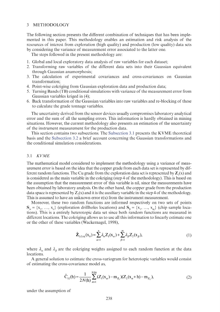
The mathematical model considered to implement the methodology using a variance of measurement error is based on the idea that the copper grade from each data set is represented by different random functions. The Cu grade from the exploration data set is represented by Z 1 (x) and
is considered as the main variable in the cokriging (step 4 of the methodology). This is based on
the assumption that the measurement error of this variable is nil, since the measurements have
been obtained by laboratory analysis. On the other hand, the copper grade from the production
data space is represented by Z 2 (x) and it is the auxiliary variable in the step 4 of the methodology.
This is assumed to have an unknown error ε(x) from the instrument measurement.
Moreover, these two random functions are informed respectively on two sets of points
S α = {x 1 , …, x n } (exploration drillholes locations) and S β = {x 1 , …, x m } (chip sample locations). This is a entirely heterotopic data set since both random functions are measured in
different locations. The cokriging allows us to use all this information to linearly estimate one
or the other of these variables (Wackernagel, 1998),
1,Cok
0
1
ˆ
(x )
Z (x )
Z (x ),
0 0
n
m
α
α
β
β
1
2
Z (x
Z (x
2
α
β
1
λ
1
1 1 1 1
∑
∑
λ Z (x )
1 1 1
Z (x )
Z (x )
1 1 1
Z
(1)
where λ α and λ β are the cokriging weights assigned to each random function at the data
locations.
A general solution to estimate the cross-variogram for heterotopic variables would consist
of estimating the cross-covariance model as,
1
2
(h)
12
1
1
1
ˆ
C (h)
(Z (x ) m )(Z (x h) m ),
2
12
1
Z
2
Z
1
Z
2
1
2 (h)
N
α
1
Z 1
Z
2
Z
2
Z
2
1
α =
(Z (x ) m )(Z (x h)
m )(Z (x h)
1
Z
2
1
Z
2
Z
2
Z
2
Z
2
∑ ∑
(2)
under the assumption of
3 METHODOLOGY
The following section presents the different combination of techniques that has been implemented in this paper. This methodology enables an estimation and risk analysis of the
resources of interest from exploration (high quality) and production (low quality) data sets
by considering the variance of measurement error associated to the latter one.
The steps followed in the present methodology are:
1. Global and local exploratory data analysis of raw variables for each dataset;
2. Transforming raw variables of the different data sets into their Gaussian equivalent
through Gaussian anamorphosis;
3. The calculation of experimental covariances and cross-covariances on Gaussian
transformation;
4. Point-wise cokriging from Gaussian exploration data and production data;
5. Turning Bands (TB) conditional simulations with variance of the measurement error from
Gaussian variables kriged in (4);
6. Back transformation of the Gaussian variables into raw variables and re-blocking of these
to calculate the grade tonnage variables.
The uncertainty derived from the sensor devices usually compromises laboratory analytical
error and the sum of all the sampling errors. This information is hardly obtained in mining
situations. However, the current methodology also presents an estimation of the uncertainty
of the instrument measurement for the production data.
This section contains two subsections. The Subsection 3.1 presents the KVME theoretical
basis and the Subsection 3.2 a brief account concerning the Gaussian transformations and
the conditional simulation considerations.
3.1 KVME
The mathematical model considered to implement the methodology using a variance of measurement error is based on the idea that the copper grade from each data set is represented by different random functions. The Cu grade from the exploration data set is represented by Z 1 (x) and
is considered as the main variable in the cokriging (step 4 of the methodology). This is based on
the assumption that the measurement error of this variable is nil, since the measurements have
been obtained by laboratory analysis. On the other hand, the copper grade from the production
data space is represented by Z 2 (x) and it is the auxiliary variable in the step 4 of the methodology.
This is assumed to have an unknown error ε(x) from the instrument measurement.
Moreover, these two random functions are informed respectively on two sets of points
S α = {x 1 , …, x n } (exploration drillholes locations) and S β = {x 1 , …, x m } (chip sample locations). This is a entirely heterotopic data set since both random functions are measured in
different locations. The cokriging allows us to use all this information to linearly estimate one
or the other of these variables (Wackernagel, 1998),
1,Cok
0
1
ˆ
(x )
Z (x )
Z (x ),
0 0
n
m
α
α
β
β
1
2
Z (x
Z (x
2
α
β
1
λ
1
1 1 1 1
∑
∑
λ Z (x )
1 1 1
Z (x )
Z (x )
1 1 1
Z
(1)
where λ α and λ β are the cokriging weights assigned to each random function at the data
locations.
A general solution to estimate the cross-variogram for heterotopic variables would consist
of estimating the cross-covariance model as,
1
2
(h)
12
1
1
1
ˆ
C (h)
(Z (x ) m )(Z (x h) m ),
2
12
1
Z
2
Z
1
Z
2
1
2 (h)
N
α
1
Z 1
Z
2
Z
2
Z
2
1
α =
(Z (x ) m )(Z (x h)
m )(Z (x h)
1
Z
2
1
Z
2
Z
2
Z
2
Z
2
∑ ∑
(2)
under the assumption of