182
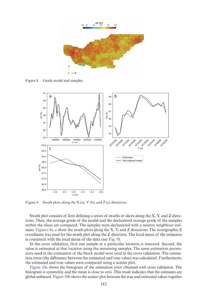
Swath plot consists of first defining a series of swaths or slices along the X, Y, and Z directions. Then, the average grade of the model and the declustered average grade of the samples
within the slices are compared. The samples were declustered with a nearest neighbour estimate. Figures 9a–c show the swath plots along the X, Y, and Z directions. The stratigraphic Z
coordinate was used for the swath plot along the Z direction. The local mean of the estimates
is consistent with the local mean of the data (see Fig. 9).
In the cross validation, first one sample at a particular location is removed. Second, the
value is estimated at that location using the remaining samples. The same estimation parameters used in the estimation of the block model were used in the cross validation. The estimation error (the difference between the estimated and true value) was calculated. Furthermore,
the estimated and true values were compared using a scatter plot.
Figure 10a shows the histogram of the estimation error obtained with cross validation. The
histogram is symmetric and the mean is close to zero. This result indicates that the estimates are
global unbiased. Figure 10b shows the scatter plot between the true and estimated values together
Figure 8. Grade model and samples.
Figure 9. Swath plots along the X (a), Y (b), and Z (c) directions.
49
~ 48
~
47
46
45
586000
50.0 c
49.5
49.0
48.5
,. i 48.0
47.5
47.0
46.5
46.0
-3.0
AA(%)
14.6 20
30
40
50
• - X
588000 590000 592000 594000
X (m\
-2.5
-2.0
-1.5
-1.0
-0.5
Z(m)
Estimates
Declustered mean