

181
4 GRADE ESTIMATION IN UNSTRUCTURED GRID
The grade estimation in the unstructured grid involves three main steps: (i) change of coordinates, (ii) variogram analysis and modeling and (iii) estimation in unstructured grid.
4.1 Change of coordinates
The Z coordinates of the data set and of the unstructured were changed to stratigraphic Z
coordinates. The stratigraphic coordinates were calculated as the Z coordinates minus the
Z coordinate of the top of the seam. The experimental variograms and estimates were performed using the stratigraphic coordinates.
4.2 Variogram analysis and modeling
The experimental variograms were calculated using the stratigraphic coordinates. The variogram model was fitted to the experimental variograms. The experimental variograms were
standardized, so the sill equals one. Equation 3 describes the variogram model of AA:
γ ( )
γ γ
,
,
.
.
.
S
)
.
.
ph
S
NS
m
EW
m
vert
m
Sph
NS
⎛
⎝ ⎜
⎛ ⎛
⎝ ⎝
⎞
⎠ ⎟
⎞ ⎞
⎠ ⎠
+
. .
60
60 1 3
. 0
0 1
. 8
700 m m
EW
m
vert
m
Sph
NS
m
EW
m
vert
m
,
,
.
.
.
,
Sph
,
.
700
8 5
.
0 1
. 0
5000
5000
9
⎛
⎝ ⎜
⎛ ⎛
⎝ ⎝
⎞
⎠ ⎟
⎞ ⎞
⎠ ⎠
+
⎛
⎝ ⎜ ⎜
⎛ ⎛ ⎛ ⎛
⎝ ⎝ ⎝ ⎝
⎞
⎠ ⎟
⎞ ⎞
⎠ ⎠
(3)
The major direction of spatial continuity is horizontal while the minor direction of spatial
continuity is vertical
4.3 Estimates in unstructured grid
The estimates were performed using ordinary block kriging. The block discretization was
5 × 5 × 1. The shape of the irregular hexahedron cells were considered to calculate the covariances
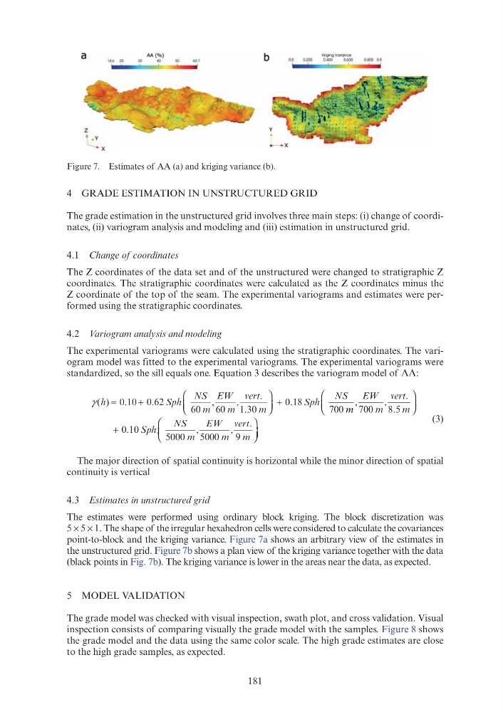
point-to-block and the kriging variance. Figure 7a shows an arbitrary view of the estimates in
the unstructured grid. Figure 7b shows a plan view of the kriging variance together with the data
(black points in Fig. 7b). The kriging variance is lower in the areas near the data, as expected.
5 MODEL VALIDATION
The grade model was checked with visual inspection, swath plot, and cross validation. Visual
inspection consists of comparing visually the grade model with the samples. Figure 8 shows
the grade model and the data using the same color scale. The high grade estimates are close
to the high grade samples, as expected.
Figure 7. Estimates of AA (a) and kriging variance (b).
a
14.6 20
• x
AA(%)
"' '
"''
b
KrlghgVoflonce
0.0
0.200
OAOO
0.600
o.&OO 0 .9
I
4 GRADE ESTIMATION IN UNSTRUCTURED GRID
The grade estimation in the unstructured grid involves three main steps: (i) change of coordinates, (ii) variogram analysis and modeling and (iii) estimation in unstructured grid.
4.1 Change of coordinates
The Z coordinates of the data set and of the unstructured were changed to stratigraphic Z
coordinates. The stratigraphic coordinates were calculated as the Z coordinates minus the
Z coordinate of the top of the seam. The experimental variograms and estimates were performed using the stratigraphic coordinates.
4.2 Variogram analysis and modeling
The experimental variograms were calculated using the stratigraphic coordinates. The variogram model was fitted to the experimental variograms. The experimental variograms were
standardized, so the sill equals one. Equation 3 describes the variogram model of AA:
γ ( )
γ γ
,
,
.
.
.
S
)
.
.
ph
S
NS
m
EW
m
vert
m
Sph
NS
⎛
⎝ ⎜
⎛ ⎛
⎝ ⎝
⎞
⎠ ⎟
⎞ ⎞
⎠ ⎠
+
. .
60
60 1 3
. 0
0 1
. 8
700 m m
EW
m
vert
m
Sph
NS
m
EW
m
vert
m
,
,
.
.
.
,
Sph
,
.
700
8 5
.
0 1
. 0
5000
5000
9
⎛
⎝ ⎜
⎛ ⎛
⎝ ⎝
⎞
⎠ ⎟
⎞ ⎞
⎠ ⎠
+
⎛
⎝ ⎜ ⎜
⎛ ⎛ ⎛ ⎛
⎝ ⎝ ⎝ ⎝
⎞
⎠ ⎟
⎞ ⎞
⎠ ⎠
(3)
The major direction of spatial continuity is horizontal while the minor direction of spatial
continuity is vertical
4.3 Estimates in unstructured grid
The estimates were performed using ordinary block kriging. The block discretization was
5 × 5 × 1. The shape of the irregular hexahedron cells were considered to calculate the covariances
point-to-block and the kriging variance. Figure 7a shows an arbitrary view of the estimates in
the unstructured grid. Figure 7b shows a plan view of the kriging variance together with the data
(black points in Fig. 7b). The kriging variance is lower in the areas near the data, as expected.
5 MODEL VALIDATION
The grade model was checked with visual inspection, swath plot, and cross validation. Visual
inspection consists of comparing visually the grade model with the samples. Figure 8 shows
the grade model and the data using the same color scale. The high grade estimates are close
to the high grade samples, as expected.
Figure 7. Estimates of AA (a) and kriging variance (b).
a
14.6 20
• x
AA(%)
"' '
"''
b
KrlghgVoflonce
0.0
0.200
OAOO
0.600
o.&OO 0 .9
I