

173
4 EXPERIMENTS
By exploring a two dimensional binary case and performing parameter sensitivities, the
RCNN approach is illustrated and a simple guide of RCNN architecture definition is
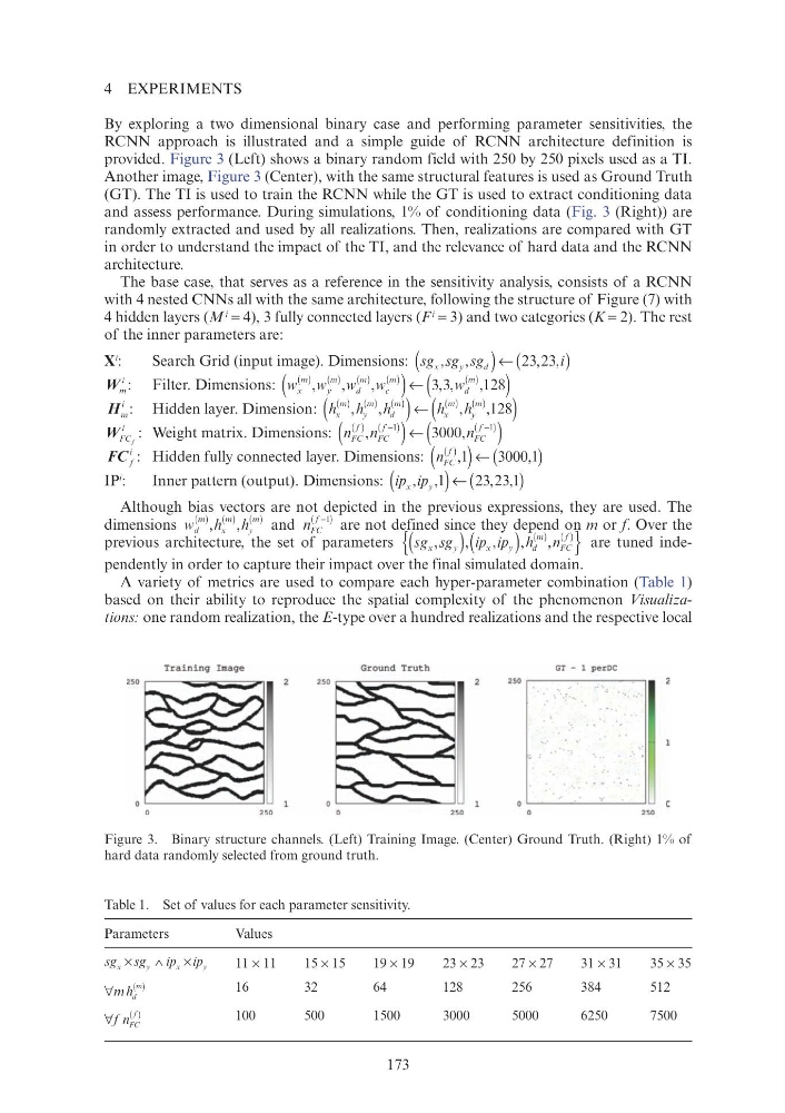
provided. Figure 3 (Left) shows a binary random field with 250 by 250 pixels used as a TI.
Another image, Figure 3 (Center), with the same structural features is used as Ground Truth
(GT). The TI is used to train the RCNN while the GT is used to extract conditioning data
and assess performance. During simulations, 1% of conditioning data (Fig. 3 (Right)) are
randomly extracted and used by all realizations. Then, realizations are compared with GT
in order to understand the impact of the TI, and the relevance of hard data and the RCNN
architecture.
The base case, that serves as a reference in the sensitivity analysis, consists of a RCNN
with 4 nested CNNs all with the same architecture, following the structure of Figure (7) with
4 hidden layers (M
i = 4), 3 fully connected layers (F
i = 3) and two categories (K = 2). The rest
of the inner parameters are:
X
i
:
Search Grid (input image). Dimensions: sg sg sg
x
y
g
d
, ,
sg y
sg
(
) ← (
)
i
, ,
W m
W W
i : Filter. Dimensions: (
)
w w w w
x
y
d
c
( )
m
( )
m
( )
m
( )
m ← (
)
w d
( )
m
w w
w w
y
d
H m
i : Hidden layer. Dimension: (
)
h h h
x
h
y
d
h
( )
m
( )
m
( )
m ← (
)
h h
x
h
y
( )
m
( )
m
h h y
h
h y
h
W FC
W W
i
f
C : Weight matrix. Dimensions: (
)
n n
FC
FC
( )
f
( )
f −
← (
)
n FC
( )
f
(
)
n FC ← (
)
) ← (
( f −
FC f
i : Hidden fully connected layer. Dimensions: ( )
n FC
( )
f
← (
)
) ← (
IP
i
:
Inner pattern (output). Dimensions: ip ip
x
y
p
, ,
ip y
ip 1
(
) ← (
)
, ,
23 2
, 3 1
,
Although bias vectors are not depicted in the previous expressions, they are used. The
dimensions w h h
d
x
y
h
( )
m
( )
m
( )
m
,
,
h x
h
and n FC
( )
f −
are not defined since they depend on m or f. Over the
previous architecture, the set of parameters {
}
y p
y p
sg sg ip ip h n
x
y
g
x
y
p
d
h
FC
,
,
sg y
sg
,
,
ip y
ip
,
(
) (
)
p p
m
f
are tuned independently in order to capture their impact over the final simulated domain.
A variety of metrics are used to compare each hyper-parameter combination (Table 1)
based on their ability to reproduce the spatial complexity of the phenomenon Visualizations: one random realization, the E-type over a hundred realizations and the respective local
Table 1. Set of values for each parameter sensitivity.
Parameters
Values
sg
ip ip
x
y
sg
x
y
ip
×
∧
sg y
sg
×
11 × 11
15 × 15
19 × 19
23 × 23
27 × 27
31 × 31
35 × 35
∀
( )
m h d
h
16
32
64
128
256
384
512
∀
( )
f n
∀ FC
100
500
1500
3000
5000
6250
7500
Figure 3. Binary structure channels. (Left) Training Image. (Center) Ground Truth. (Right) 1% of
hard data randomly selected from ground truth.
Tra i n i ng I mage
Gr o u n d Truth
GT - 1 p e r DC
2 5 0
250
250
250
4 EXPERIMENTS
By exploring a two dimensional binary case and performing parameter sensitivities, the
RCNN approach is illustrated and a simple guide of RCNN architecture definition is
provided. Figure 3 (Left) shows a binary random field with 250 by 250 pixels used as a TI.
Another image, Figure 3 (Center), with the same structural features is used as Ground Truth
(GT). The TI is used to train the RCNN while the GT is used to extract conditioning data
and assess performance. During simulations, 1% of conditioning data (Fig. 3 (Right)) are
randomly extracted and used by all realizations. Then, realizations are compared with GT
in order to understand the impact of the TI, and the relevance of hard data and the RCNN
architecture.
The base case, that serves as a reference in the sensitivity analysis, consists of a RCNN
with 4 nested CNNs all with the same architecture, following the structure of Figure (7) with
4 hidden layers (M
i = 4), 3 fully connected layers (F
i = 3) and two categories (K = 2). The rest
of the inner parameters are:
X
i
:
Search Grid (input image). Dimensions: sg sg sg
x
y
g
d
, ,
sg y
sg
(
) ← (
)
i
, ,
W m
W W
i : Filter. Dimensions: (
)
w w w w
x
y
d
c
( )
m
( )
m
( )
m
( )
m ← (
)
w d
( )
m
w w
w w
y
d
H m
i : Hidden layer. Dimension: (
)
h h h
x
h
y
d
h
( )
m
( )
m
( )
m ← (
)
h h
x
h
y
( )
m
( )
m
h h y
h
h y
h
W FC
W W
i
f
C : Weight matrix. Dimensions: (
)
n n
FC
FC
( )
f
( )
f −
← (
)
n FC
( )
f
(
)
n FC ← (
)
) ← (
( f −
FC f
i : Hidden fully connected layer. Dimensions: ( )
n FC
( )
f
← (
)
) ← (
IP
i
:
Inner pattern (output). Dimensions: ip ip
x
y
p
, ,
ip y
ip 1
(
) ← (
)
, ,
23 2
, 3 1
,
Although bias vectors are not depicted in the previous expressions, they are used. The
dimensions w h h
d
x
y
h
( )
m
( )
m
( )
m
,
,
h x
h
and n FC
( )
f −
are not defined since they depend on m or f. Over the
previous architecture, the set of parameters {
}
y p
y p
sg sg ip ip h n
x
y
g
x
y
p
d
h
FC
,
,
sg y
sg
,
,
ip y
ip
,
(
) (
)
p p
m
f
are tuned independently in order to capture their impact over the final simulated domain.
A variety of metrics are used to compare each hyper-parameter combination (Table 1)
based on their ability to reproduce the spatial complexity of the phenomenon Visualizations: one random realization, the E-type over a hundred realizations and the respective local
Table 1. Set of values for each parameter sensitivity.
Parameters
Values
sg
ip ip
x
y
sg
x
y
ip
×
∧
sg y
sg
×
11 × 11
15 × 15
19 × 19
23 × 23
27 × 27
31 × 31
35 × 35
∀
( )
m h d
h
16
32
64
128
256
384
512
∀
( )
f n
∀ FC
100
500
1500
3000
5000
6250
7500
Figure 3. Binary structure channels. (Left) Training Image. (Center) Ground Truth. (Right) 1% of
hard data randomly selected from ground truth.
Tra i n i ng I mage
Gr o u n d Truth
GT - 1 p e r DC
2 5 0
250
250
250